Team B3: 2D23D

This week I have been implementing the point cloud generation algorithm for the simulated 3D scan. This has involved snooping around the blender and writing simple scripts to extract the data relevant to transformations between the different spaces of our algorithm. For example, while it is not displayed directly on the UI, blender keeps track of transformations from the local space of each object to the space of its parent. So by writing a script like the following:

We were able to extract a transformation matrix (4×4 for a 3d vector, including translation, scale, and rotation) converting points in the coordinate space of the laser line to world space. By using this, we can simply get an equation for the laser plane by applying this transformation to a very simple vector (1,0,0,1). Similar scripts were written to extract camera transform data, which was used to implement the transformation of pixels in the image to world space.

The two major elements that are written so far are:

1. The detection of laser pixels in an image
2. The transformation of screen pixels to corresponding points in world space

A rough version of laser pixel detection was implemented last week, but this week I was able to optimize it to run in a fraction of the time it took earlier. I have also set the maximum number of laser pixels to detect per row to 3, so that there are not too many excess points being added to the point cloud. The code right now is below:

Transformations from pixels to screen points is then implemented in two steps:

1. Convert pixels to camera space
2. Transform camera space positions to world space

Step 1 is implemented by using the perspective camera model, with a known focal point and sensor dimensions from the blender file used during the simulation. Step 2 is implemented by applying the inverse transform of the camera onto the points of the sensor. The code is below:

The next steps to complete are ray-plane intersection to get the position of those pixels projected on the object in world space, and finally reverse rotation to get the same points in object space. After this, we will have completed the pipeline for a single scan. I plan to have this completed by our team meeting on Monday. Hopefully, a full example scan will be able to be completed by this time.

Right now, I believe the work is ahead of schedule, and a working demo will be available early next week. Because of the extra slack time this provides us, we may work on adding additional features for our demo, such as a web application GUI.

This week I continued working on simulating the data we would get for the laser projection. I tweaked a few parameters and also got the animation to work. Now, Blender can either render a whole video or render a bunch of images with each frame of the video being saved as an image instead. We will use the set of images with a known rotation angle shift per image (360 degrees / number of frames) as input to our scanning software.

Here is the video of the rotating laser scan, where the laser is projecting from the right side: https://youtu.be/7rv-rFpyDcM

I updated the block diagram for our system – note that all the physical components have been removed, and the controllers are also removed. We have Blender-simulated data instead for the input, and we will likely use a Django web app for ease of running Python with a simple web interface rather than using some Python GUI like Tkinter which would take more unnecessary time to implement. Chakara and I are both experienced in developing web applications so using Django is more of a choice of saving time in a portion that isn’t entirely essential to the project. 

Moving forward, I will finalize the laser scan by adding a platform and also calibrating the angle between the camera and the laser, as well as the height of these two items. I will also start finding more objects that fit our project, and will look to start implementing some of the code to perform outlier removal on the point cloud.

As mentioned in the team status update, we are switching our project to simulate or generate images that we would normally get from the camera and laser setup instead of building a physical piece of hardware. I started to explore options to do this, and I will be using Blender modeling software to generate these images. In these few days, I successfully projected a laser stripe onto the default Blender object Susanne the monkey. 

 

This is a sample of the laser stripe projected onto the object. I will add a cylindrical platform with a wood texture and tune the background to be dark grey or something so we can see the laser better. 

 

 

This is the shading setup I used for the laser projection. I used an image with a white line of a few pixels wide down the middle and actually projected the image shaded with a red tint to resemble a laser stripe. I can tune how white or red the laser stripe is with the power parameter in Blender (set to 70,000W in the render above). I can also control how much red diffuses from the laser by tuning how many light bounces there will be in the render. 

 

Moving forward, I will be using keyframe animations to rotate an object around the z-axis and generate images resembling what we would get in our physical setup. I will need to first acquire our old materials from Quinn so I can assemble a basic non-moving version of our previous design to check how well my simulated images resemble it, and also get the camera parameters of our USB camera to calibrate those in Blender.

Since we have decided to transition our project from a physical device to a proof-of-concept simulation due to the COVID-19 circumstances, some changes must be made to the 3D scanning algorithm. Most notably, since there is no hardware and physical uncertainties to worry about, such as lighting conditions, vibrational noise, strange object materials, a large part of our calibration procedure can be skipped entirely. Actually, the entire calibration procedure can be skipped, since we know parameters directly from how we set up a simulated scan. A run down of the calibration parameters and where they come from:

1. Intrinsic Camera – These parameters are related to the curvature of the lens and influence the polynomial transformation between a projection onto the camera, and an image pixel coordinates. We can set this transformation to the identity function on the simulation to simplify the whole process.
2. Extrinsic Camera – The transformation between camera space and turn-table space is given by the relative position of the camera in relation to the turn-table, which is known in the simulation.
3. Turntable Axis of Rotation – This is based on where we place the turntable in simulated space, so it is known.
4. Laser-Plane – This is based on the position and angle of the lazer line source in relation to the turn-table origin, which is known.
5. Rotational Angle – This is accurately changed by the simulation for each frame captured, so this is known as well.

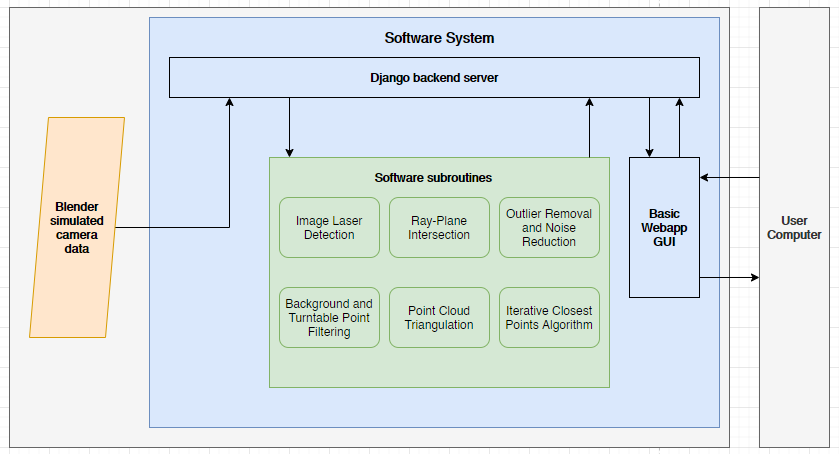
Because of the ease of specifying parameters for the simulation, none of these parameters need to be calibrated for, and can simply be specified when starting the simulation. Because of this, a large amount of the complexity in our algorithm is immediately gone when switching to a simulation. The only remaining major step is to write code to implement the main 3D scanning pipeline:

1. Image Laser detection – Note that the laser line can have a perfect gaussian intensity distribution along its width, so there is no need for the additional filter in software.
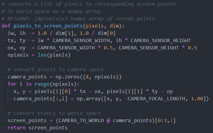
2. Generate ray from camera source through pixel in world space
3. Ray-Plane intersection to find position on the laser plane
4. Reverse rotation about turntable axis to find position in object space
5. Aggregate found points to point cloud

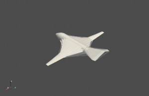
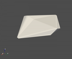
After this is done, routines can be implemented for mesh triangulation from the point cloud, and we have completed the scan. We will be aiming to complete this simple pipeline before allocating any time towards single-object multiple-scan or other complex features. Since our ground-truth meshes are now completely reliable (since they are the absolute source of data from the simulation), verification will be much easier to implement. We will implement the full pipeline before any verification steps to ensure that qualitatively our solution works. Then we will optimize it to meet our accuracy requirements. We will no longer worry about end-to-end timing requirements for this project, since there is no longer a physical device. However, we will ensure that our software components (not including the simulation, which may take a while to capture data due to the complexities of simulating lighting and rendering), take under a minute for a full scan.

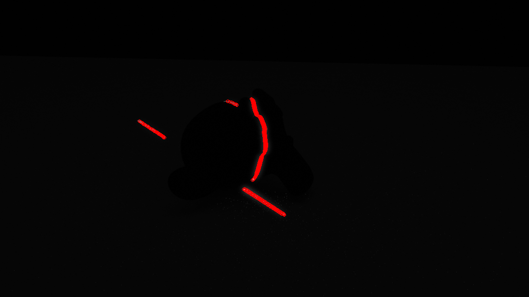
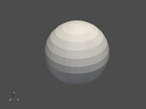
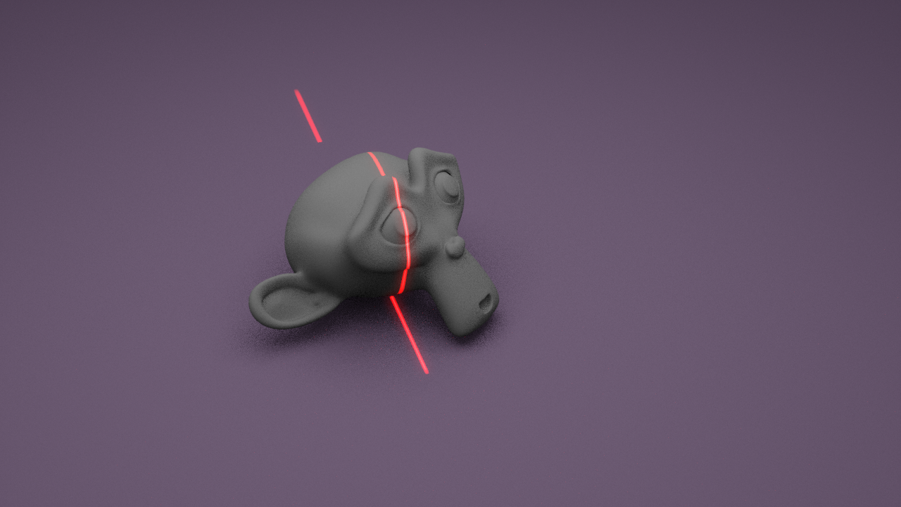
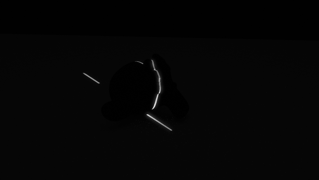
I have been working on writing the prototype code for image-laser detection. Our original plan was to only detect a single point with maximum intensity for each row of pixels. However, this poses a problem with the following image:

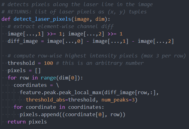
This is clearly a reasonable image during a scan, however a single row of pixels may contain 2 or even 3 instances of the laser line! To alleviate this problem, in my prototype code I have found all local maxima along the row of pixels above some arbitrary intensity threshold (this threshold can be fine-tuned as we gather more data). First, the code applies a filter to the image to extract red intensity, which is computed for each pixel as:

max(0, R – G/2 – B/2)

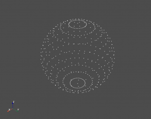
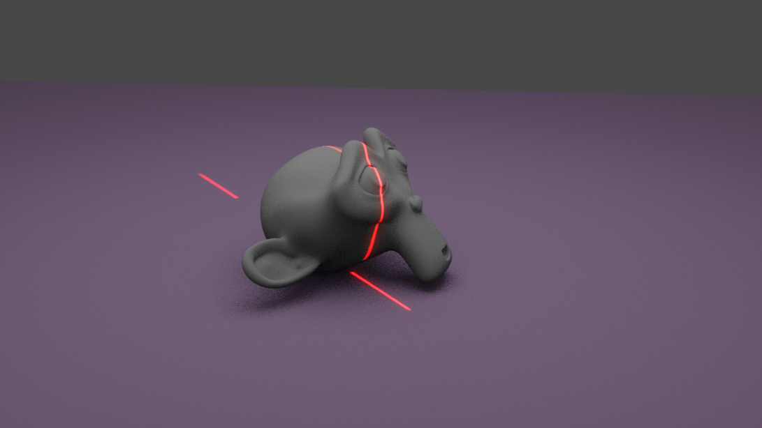
Where R, G, and B are the red, blue, and green channels of the pixel respectively. Since a 650nm laser line corresponds directly to the color RGB(255,0,0), we only need to worry about the red component. The filtered image is:

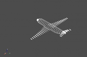
Finally, after laser line detection (where each point detected is circled in red), we have the following points to add to the point cloud after transformations:

No status report due to spring break and emergency actions taken because of COVID-19.

This week, our team received the mechanical parts and started testing a few of the components. Currently, our risk is similar to last week’s which is mainly the motor and jetson integration, but we already talked to Professor Nace and we could check if Quinn has an extra Arduino. Thus, this risk is mitigated. Our parts also came in time and most of them worked as we expected. There were no changes being made to the existing design of the system yet.

 

This is the link to our updated schedule: https://docs.google.com/spreadsheets/d/1GGzn30sgRvBdlpad1TIZRK-Fq__RTBgIKN7kDVB3IlI/edit?usp=sharing