Team B3: 2D23D

During this week we had a breakthrough moment for the project. Instead of choosing a sensor by what we thought would be interesting, we got detailed, quantitative requirements for the sensor so it became easy to choose.

We started from our requirements. In the most extreme case, to accurately capture an object whose longest axis is 5cm, in order to meet the requirement that 90% of reconstructed points are within 2% of that 5cm, we must have points within 1mm to the ground truth model. From this, if we consider the number of samples we need across the surface, we must have accurate samples within 1mm for each direction (X, Y along the surface). Since the surface itself is a continuous signal we are sampling from, we can compute the Nyquist sampling rate as being every 0.5mm along each direction of the surface. 

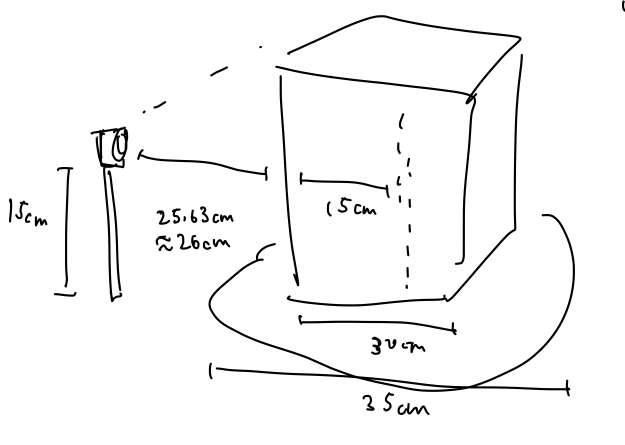
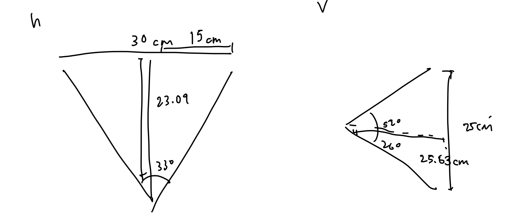
Now considering the rotational mechanism, the largest radius of the object from the center of the rotating platform will be within 15cm. We need then a single rotation per data capture to be such that the amount of the surface rotated passed the sensor is less than or equal to 0.5mm. This gives us a 0.5mm / 150mm = 0.0033 radians of rotation per sample.

There are five main types of depth sensors applicable to 3D scanning available that we have deeply considered:

1. Contact sensors, widely used in manufacturing. A Coordinate Measuring Machine (CMM) or similar may be used, which generally utilizes a probing arm to touch the sensor, and through angular rotations of the joints the coordinates of each probed area can be computed. This is a non-option for our application, both for price and the fact that we should not allow a large machine to touch timeless archeological artifacts.
2. Time-of-flight sensors. By recording the time between sending a beam of light and receiving a reflected signal, distance can be computed to a single point. The disadvantage of this approach is that we can only measure times so precisely, and the speed of light is very fast. With a timer that has 3.3 picosecond resolution, we are still not within sub-millimeter depth resolution, which is not reasonable for this project. Time-of-flight sensors in the domain of 3D scanning are more applicable to scanning large outdoor environments.
3. Laser triangulation sensors. The principle of such a sensor is that an emitting diode and corresponding CMOS sensor are located at slightly different angles of the device in comparison to the object, so depth can be computed by the location on the sensor the laser reflects to. Generally the position of the laser on the surface is controlled by a rotating (or pair of rotating) mirrors (https://www.researchgate.net/publication/236087175_A_Two-Dimensional_Laser_Scanning_Mirror_Using_Motion-Decoupling_Electromagnetic_Actuators). Assume that such a sensor is affordable, can easily measure with resolution of less than 0.5mm, and we do not encounter any mechanical issues. The total number of distance measurements we are required to record is (2pi / 0.0033)  * (300mm / 0.5mm) = 1142398 by our calculations above. Assuming the sensor has a sampling rate of about 10khz (common for such a sensor), 1142398 points / 10000 points per second = 114.23 seconds theoretical minimum capture time with one sensor. From our timing requirement, assume that half of our time can be attributed to data collection (30 seconds). Then, with perfect parallelization, we could achieve our goals with 114.23s / 30s = 3.80 = 4 sensors collecting concurrently. With our budget, this is not achievable. Even if we had the budget, it is possible for systematic errors in, for example, the mounted angle of a sensor, to propagate throughout our data with no course for resolution. To add another set of sensors to mitigate this error, we would be even farther out of our budget. 8 sensors * $300 per sensor (low-end price) = $2400. Note these calculations are unrelated to any mechanical components, but are directly derived from required data points. To make budget not an issue, we could choose to adopt cheaper sensors, such as those with under 1khz sampling rate. Performing the same calculations as above with 1khz sampling rate shows us that we would require 39 sensors to meet our timing requirement, which is well out of the realm of possibility (and this is not accounting for error-reduction, which may require 78 sensors!). If we did not purchase this amount of sensors, we would drastically under perform for our timing requirement. Of course, there is an alternative to single-point laser triangulation. We may use a laser stripe depth sensor, which gets the depth for points along a fixed width stripe (https://www.researchgate.net/publication/221470061_Exploiting_Mirrors_for_Laser_Stripe_3D_Scanning). This would improve our ability to meet our timing requirements significantly. Such devices are not easily available with high accuracy to consumers, but are usually intended for industry and manufacturing. Because of this, we would have the responsibility of constructing such a device. We have considered the risk of building our own sensor, and since none of our team members are experts in the fields of sensors and electronics, there is a high potential for error on the accuracy of a constructed laser stripe depth sensor. However, we are up to the task. A stripe laser sensor consists of the pair of a projected linear light source and a CCD camera. After a calibration process to determine the intrinsic camera parameters as well as the exact angle and distance between the camera and the laser projector, linear transformations may be applied to map each point from screen space to world space coordinates. Generally the issue here, even if we do construct a perfect laser stripe depth sensor, is that micro-vibrations from the environment may introduce significant jitter in the data acquisition process. Because of this, laser sensors for 3D reconstruction are generally done in tandem with alternative sources of information, such as a digital camera or structured light depth sensor, to minimize vibrational error (https://www.ncbi.nlm.nih.gov/pmc/articles/PMC4279470/#b8-sensors-14-20041). An alternative solution is to add an additional stripe laser sensor (https://www.sciencedirect.com/science/article/pii/S1051200413001826), which would help eliminate such errors. Because of the ease of achieving sub-millimeter accuracy, and the relative independence on lighting conditions and materials that photogrammetry is harmed by, we plan on constructing a laser stripe triangular depth sensor by using an CCD camera.
4. Digital camera. By taking multiple digital photographs from many perspectives around the object, computer vision techniques can be used to match features between pairs of images, and linear transforms can be computed to align such features. After feature alignment, and depth calculation, point clouds can be generated. Computer vision techniques to accomplish the above include Structure from Motion (SfM) and Multi-View Stereo reconstruction (MVS) (http://vision.middlebury.edu/mview/seitz_mview_cvpr06.pdf). This approach has a fundamental flaw: concavities in the object to be scanned cannot be resolved, since cameras do not capture raw depth data. Surface points within the convex hull of an object cannot be easily distinguished from points on the convex hull. This is an immediate elimination for our project, since archeological objects may have concavities, and we do not want to limit the scope of what type of objects can be captured.
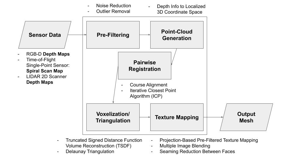
5. Structured/coded light depth sensor (RGB-D Camera). The idea of such a sensor is to project light in specific patterns on the object, and compute depth by the distortion of the patterns. Such sensing devices have become incredibly popular in the 3D reconstruction research community with the consumer availability of the Microsoft Kinect (https://www.researchgate.net/publication/233398178_Kinect_and_RGBD_Images_Challenges_and_Applications). The original Microsoft Kinect only has 320 pixels wide of depth information for a single depth image. With the upper bound of 30cm across the surface of the object, this results in 30cm/320px = 0.094cm between each pixel, which does not meet our sensor requirement of being able to detect differences within 0.5mm (0.05 cm). The newer Microsoft Kinect v2 actually uses a time-of-flight sensor, and thus does not get measurements more accurate than 1mm depth resolution. Intel RealSense has recently released new product lines for consumer and developer structured light depth sensors, that do not require industrial/manufacturing budgets. Most notably, for short range coded light depth sensing, the Intel RealSense SR305 offers 640×480 pixel depth maps, which correlates to 30cm/640px = 0.047cm, which is within our requirements. If vertical accuracy becomes a problem with the 480px, we can rotate the camera up or utilize a mirror to take two captures for each perspective. Ensuring that the capture of the camera covers most of the object, we need about 30cm distance with its minimum 66 degree horizontal camera angle, and 52 degree vertical. This works well with the camera’s minimum depth capture of 20cm. Finally, with structured light depth sensing, depth resolution is somewhat proportional to distance, so as long as our object is close to the sensor, we would hopefully achieve sub-millimeter depth resolution. Intel does not advertise any specific depth resolution for the device. We would need to perform extensive testing to discover actual depth accuracy before further implementation. Lighting environment and material of the object can also influence depth resolution, which we will investigate with a variety of objects. Compared to laser triangulation, in which most of the effort is up-front in sensing devices and mechanical components, structured light depth sensors require a significant algorithmic effort after data collection to correlate the views. We have already designed an algorithmic pipeline to go from multiple depth maps, to localized point clouds, to a global point cloud, to a triangular mesh. This heavy computation must meet our timing requirement of one minute, so we will be programming the algorithms from scratch to run on the GPU of the embedded system for the device.

A summary of our extensive sensor research this week: we have eliminated the options of contact sensors, time-of-flight sensors, and digital cameras. Both laser triangulation sensors and structured light depth sensors have promise. Because of the potential for vibrational and mechanical error for the laser triangulation sensor, we would likely need to use it in tandem with another laser triangulation sensor. As much as purchasing the Intel SR305 would speed up our development time, we do not know if it actually has sub-millimeter accuracy, which is a requirement, and as a product our project may be more cost effective if we build a laser triangulation sensor with two stripes and a CCD camera (depending on the cost of the CCD camera we may choose to buy a CMOS one instead).

Because of this, we will begin by searching for and buying a CCD camera, as well as two laser stripe projectors. From this we can begin implementing our calibration routines and discovering the accuracy of the scanner. We are mostly interested in the accuracy of the calibration routine, which will tell us the intrinsic parameters of the camera, which can be verified, and will also tell us computed distances and angles between the camera and the laser stripes, which can also be verified.

Next, we need to consider how we will evaluate the metrics and validation of our design. There are several components to the pipeline, and we will unit test each component individually, and integration test our final project’s results.

For accuracy of our sensor setup, we will verify the calibration procedure as mentioned above. We can also use early generated point clouds to determine standard deviation from plane fit, normalized RMS, the subpixel accuracy, distance accuracy and fill rate. From these values, we will be most interested in a sub-millimeter Z-accuracy, which is computed as the median of differences in depths to the actual distance of the plane. If the sensor does not achieve this goal, we may be forced to add an additional RGB-D camera to aid in data collection.

For accuracy of our software, we will write a simple sequential version of the code and ensure that for each stage of the pipeline, our results from the GPU-accelerated code match.

For accuracy of our rotating platform, we will measure that each step of rotation for the motor is equal to or less than our intended rotation of 0.0033 radians. 

For verification of our project as a whole, we will test each of the requirements. Timing can be measured by stopwatch, and price can be measured by our order receipts. Accuracy will be a mix of using known objects such as coke bottles and measured cubes, and 3D printed archeological objects, for which we will allow an excess 1mm accuracy violation due to the inconsistencies of 3D printing.

This week I spent time researching the common pipeline generally utilized in 3D Mesh reconstruction from raw depth data. The core of the pipeline is the Pairwise Registration stage, which aims to join localized point clouds from each perspective into a global 3D coordinate space. A common technique to accomplish this is the Iterative Closest Point (ICP) algorithm, which estimates the rotation between two subsequent views of depth information, and continuously iterates on this value until relative points line up with a low mean squared error cost. Once the rotations have been computed between relative views, rotational matrices can be applied to each view to transform them into a global coordinate space, thus achieving a final point cloud. It is possible for us to provide an initial estimate for the rotation by capturing data from our rotational mechanism, but we will still utilize an iterative approach, since this initial recording may not be accurate with the depth info collected.

Problems with ICP include: time complexity is quadratic in number of points, since each pair of points is considered (Oct-tree or similar data structure can get this to O(nlogn)); some points may not have corresponding points in the subsequent view; if two views are at far enough angles, the algorithm can be trapped in a local minimum. Many variants of the ICP algorithm exist, which select points from each view, match points between the views, weight pairs of points between the views, and define error metrics differently. These decisions are aimed to eliminate systematic biases in our system which may result in the algorithm being stuck in a local maximum. For example, if our sensor captured RGB data with each depth point, matching points can be biased with this information, likely resulting in an algorithm that will match correct points more often. We prioritize accuracy more than we do performance, based on our stated project requirements during our project proposal. Because of this, our choice in a variant of the ICP algorithm will be based on avoiding local minima which will skew the accuracy of our final point cloud. From this we are pushed to make our rotational mechanism rotate a small angle between views, and possibly make our sensor capture RGB data for ease of point matching.

Other steps which we will also need to consider are pre-filtering and point-cloud generation for each view. These steps are largely dependent on the sensor data we receive, and thus are dependent on the devices we choose to capture the data, which Jeremy has done research in this week. Finally, mesh construction from the point cloud and optional (stretch goal) texture mapping must be done to form a usable 3D format for the user. We must choose a format for the output mesh (volume-based or triangular surface mesh), and then choose a corresponding algorithm appropriately. Triangular surface meshes are more generally usable by more software, so if we choose a volumetric approach, we may utilize a public library to triangulate the result. It will be easier to directly implement the construction of a volumetric mesh from point-cloud data, so for the sake of time (and not re-inventing the wheel of triangulation algorithm implementations), we will most likely choose this approach.

Below is a general diagram of our initial algorithmic pipeline. Much of the details need to be sorted out based on our data collection mechanism. Our ability to provide texture mapping is also dependent on whether our sensor captures RGB data.

Algorithmic Pipeline Diagram

In terms of developing our algorithmic approach, we are on the schedule set by our Gantt chart. In the next week we will have chosen a specific sensor approach, which will enable us to narrow in on our pre-filtering and point-cloud generation techniques. By this point we will also be able to choose a variant of the ICP algorithm for pairwise registration based on foreseen metric trade-offs. Finally, with our sensor chosen, we can determine whether or not we will be able to perform texture mapping as a stretch goal. At the end of next week, after our algorithmic pipeline has been determined to a large degree, we can plan the specific technologies we will utilize to implement each stage.

As of now to manage risk, we are choosing techniques general enough that regardless of sources of error from the sensor side, we can accommodate by adding an additional filtering step during pre-processing. This is, of course, assuming the sensor data does not have egregiously high noise.