This week I spent time researching the common pipeline generally utilized in 3D Mesh reconstruction from raw depth data. The core of the pipeline is the Pairwise Registration stage, which aims to join localized point clouds from each perspective into a global 3D coordinate space. A common technique to accomplish this is the Iterative Closest Point (ICP) algorithm, which estimates the rotation between two subsequent views of depth information, and continuously iterates on this value until relative points line up with a low mean squared error cost. Once the rotations have been computed between relative views, rotational matrices can be applied to each view to transform them into a global coordinate space, thus achieving a final point cloud. It is possible for us to provide an initial estimate for the rotation by capturing data from our rotational mechanism, but we will still utilize an iterative approach, since this initial recording may not be accurate with the depth info collected.
Problems with ICP include: time complexity is quadratic in number of points, since each pair of points is considered (Oct-tree or similar data structure can get this to O(nlogn)); some points may not have corresponding points in the subsequent view; if two views are at far enough angles, the algorithm can be trapped in a local minimum. Many variants of the ICP algorithm exist, which select points from each view, match points between the views, weight pairs of points between the views, and define error metrics differently. These decisions are aimed to eliminate systematic biases in our system which may result in the algorithm being stuck in a local maximum. For example, if our sensor captured RGB data with each depth point, matching points can be biased with this information, likely resulting in an algorithm that will match correct points more often. We prioritize accuracy more than we do performance, based on our stated project requirements during our project proposal. Because of this, our choice in a variant of the ICP algorithm will be based on avoiding local minima which will skew the accuracy of our final point cloud. From this we are pushed to make our rotational mechanism rotate a small angle between views, and possibly make our sensor capture RGB data for ease of point matching.
Other steps which we will also need to consider are pre-filtering and point-cloud generation for each view. These steps are largely dependent on the sensor data we receive, and thus are dependent on the devices we choose to capture the data, which Jeremy has done research in this week. Finally, mesh construction from the point cloud and optional (stretch goal) texture mapping must be done to form a usable 3D format for the user. We must choose a format for the output mesh (volume-based or triangular surface mesh), and then choose a corresponding algorithm appropriately. Triangular surface meshes are more generally usable by more software, so if we choose a volumetric approach, we may utilize a public library to triangulate the result. It will be easier to directly implement the construction of a volumetric mesh from point-cloud data, so for the sake of time (and not re-inventing the wheel of triangulation algorithm implementations), we will most likely choose this approach.
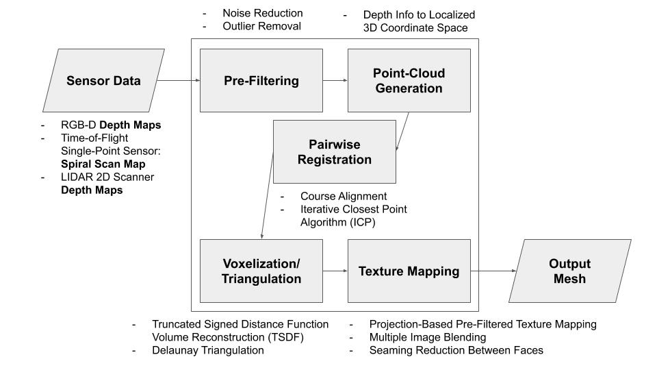
Below is a general diagram of our initial algorithmic pipeline. Much of the details need to be sorted out based on our data collection mechanism. Our ability to provide texture mapping is also dependent on whether our sensor captures RGB data.
Algorithmic Pipeline Diagram
In terms of developing our algorithmic approach, we are on the schedule set by our Gantt chart. In the next week we will have chosen a specific sensor approach, which will enable us to narrow in on our pre-filtering and point-cloud generation techniques. By this point we will also be able to choose a variant of the ICP algorithm for pairwise registration based on foreseen metric trade-offs. Finally, with our sensor chosen, we can determine whether or not we will be able to perform texture mapping as a stretch goal. At the end of next week, after our algorithmic pipeline has been determined to a large degree, we can plan the specific technologies we will utilize to implement each stage.
As of now to manage risk, we are choosing techniques general enough that regardless of sources of error from the sensor side, we can accommodate by adding an additional filtering step during pre-processing. This is, of course, assuming the sensor data does not have egregiously high noise.