Author: acpatel

Over the course of this last week, I worked on helping with Jeremy’s final presentation (Sunday – Monday), then began generating some clips for the video demo. I generated both audio recordings of myself explaining the components I worked on in the implementation, as well as some screen recorded clips demonstrating the concepts I discuss. Finally, for the video, I created a blender animation of the monkey mesh being unearthed from the sand, which was a good learning experience in 3D rendering and animation for me.

Jeremy worked hard and managed to create a very well produced video for our project, arranging many components in a cohesive story. We all gave him copious feedback to improve the video, and then starting Friday, we began working on our final report. I am now working on assembling additional figures to demonstrate the validation plan that has become more concrete since our Design Review Presentation. Namely, we have been using a dataset of several 3D ground truth meshes acquired via Sketch Lab from two primary sources (these sources will be cited in our report). These sources provide real scanned archaeological objects, so meet our user story exactly. Also since the design review report, we have created quantitative metrics with which to asses the accuracy of scans in multiple ways. I will continue to generate data and add these figures to the final report.

I am currently on schedule, do not foresee any major risks, and plan to help finish the final report by the deadline.

This week was really focused on wrapping up the pipeline into a complete package that is “shippable”. We still have a few things to add to allow other people to use it, such as a README.md explaining how the software works and how people can perform scans of their own, and the report explaining the design, metrics, and tradeoffs that went into the development of our project. All of these things will be completed next week in time for the report and video submissions.

This last week, I have mainly been working on updating the verification module to allow us to gather sufficient data to present for our final presentation. We wanted to weigh each design tradeoff we made by using quantitative results, so we updated the driver script as well as the verification engine to produce more data that we could capture as csv files (usable files in excel).

The main new metric we came up with is the notion of scan “Accuracy”, whose formula directly follows our accuracy requirement for the project.

1. 90% of vertices of our reconstructed object must be within 2% of the longest axis of the ground truth mesh to the ground truth mesh.
2. 100% of vertices of our reconstructed object must be within 5% of the longest axis of the ground truth mesh to the ground truth mesh.

We noticed that while this is a good metric for accuracy of our scan, it does not paint a complete picture. We are missing the idea of “completeness”, which is how much of the ground truth mesh is covered by our reconstructed mesh. This data is captured by taking the same formulation as our requirements above, but reversing the roles of the reconstructed mesh and the ground truth mesh (that is testing how close vertices of the ground truth mesh are to our reconstructed object, if this is high then our reconstructed object “completely” fills the space the ground truth mesh did). We encode these two ideas, of accuracy and of completeness, by the notation “forward” and “backward” accuracy.

Now that we have made this distinction, it is important to note that forward accuracy is the only important metric to our requirements: we are only truly concerned about the accuracy of the points we generate. However, the notion of completeness was used to weigh some of our design tradeoffs, so it is important to include. Below is the final formulation of general accuracy (which applies to both forward, backward, and “total” accuracy).

• accuracy = 100% – 0.9 * (% points farther than 2% but closer than 5%) – (% points farther than 5%)

In a sense, this formulation of accuracy conveys our requirement while providing a numeric representation of our results. When determining total accuracy for a reconstructed mesh, we compute both forward and backward accuracy and average them weighted by number of vertices on the ground truth/reconstructed mesh.

I implemented the data processing required to capture the accuracy data in the verification engine, and we have recently utilized this data to construct graphs and figures to demonstrate the tradeoffs we have made during the project. Right now I believe we are on schedule, since we are prepared for the final presentation. There are currently no significant risks to report. As noted earlier, we plan to make a “shippable” version next week as well as work on the videos and the final report.

At the start of this week I had completed implementing the point cloud generation algorithm, and now with both ICP completed by Jeremy for single-object multiple-scans and mesh triangulation completed by Chakara, I could begin writing a program to verify our accuracy requirement on simulated 3D scans. 

Our accuracy requirement is as follows: 90% of non-occluded points must be within 2% of the longest axis to the ground truth model. 100% of non-occluded points must be within 5% of the longest axis to the ground truth model.

The first thing to do is to figure out how to find the distance between scanned points and the ground truth mesh. This is done by utilizing the ICP algorithm we already implemented to align the mesh. The procedure is as follows:

1. Sample both the scanned mesh and the ground truth mesh uniformly to generate point clouds of their surfaces.
2. Iterate ICP to generate a transformation matrix from the scanned mesh to the ground truth mesh.
3. Apply the transformation to each vertex of the scanned mesh to align it to the same rotation/translation as the ground truth mesh.

The need for this alignment is that the ground truth mesh can be oriented differently than our scanned copy, and before we can evaluate how different the meshes are they must be overlaid on each other. The following image is a demonstration of the success of this mesh alignment:

Here the grey represents the ground truth mesh, and the white is the very closely overlaid scanned mesh. As you can tell the surface triangles weave in and out of the other mesh, so they are quite closely aligned.

Now that both meshes are aligned, we need to compute the distance of each vertex of the scanned mesh to the entirety of the ground truth mesh. The algorithm is as follows to compute the distance of a point to a mesh:

1. For each vertex of the scanned mesh
   1. For each triangle of the ground truth mesh
      1. Determine the distance to the closest point of that triangle
   2. Determine the minimum distance to the ground truth mesh out of all the triangles
2. Determine the number of distances farther than 2% of the longest axis
3. Determine the number of distances farther than 5% of the longest axis
4. If the number of distances farther than 2% of the longest axis is more than 10% (100% – 90%) of the number of points, accuracy requirement has failed
5. If any distances are farther than 5% of the longest axis, accuracy requirement has failed.
6. Otherwise, verification has passed successfully, and accuracy requirements are met for the scan. Note that occlusion points are not considered since they can be accounted for by performing single-object multiple-scans using ICP.

This looks good, but the double for loop incurs a significant performance cost. We are ignoring this cost since the speed of verification is not important to any of our requirements (this cost can be alleviated by the use of a kd-tree or similar to partition the triangles into a hierarchy).

Finally, we are left with the question of how we can determine the distance of a point to the closest point on a triangle. The procedure to do this is to project the point onto the plane of the triangle, then determine which region of the triangle the point is in on the plane, and finally based on that region perform the correct computation. The regions are illustrated below for the 2D case:

The computation is as follows for each of these cases:

1. Inside the triangle, the point distance is the distance from the point to the plane
2. To the line segment, the distance is the hypotenuse of the distance to the plane and the distance from the point on the plane to the line segment. This distance is computed by subtracting the portion of the vector from the projected point to a vertex that is parallel to the segment.
3. To a point of the triangle, the distance is the hypotenuse of the distance to the plane and the distance from the point on the plane to the point of the triangle.

There were a couple implementation hurdles, such as figuring out how to extract triangle data from the mesh object. Specifically, the triangles property is an array of 3-tuples where each element corresponds to an index to a vertex in the vertices array. In this way triangles can be reconstructed by utilizing both of these arrays. Below is a sample of code to perform the distance computation from a point to a mesh, the point to triangle computation is quite complicated and is not posted here:

With all of this now implemented, we can perform verification of our scans to check that they meet the accuracy requirements. However, this verification process takes a significant amount of time, so I may in the next week optimize it to use a tree data structure.

My part of the project is on schedule for now, and at this moment we are preparing some examples for our in-lab demo on Monday. This next week I hope to optimize the verification process, test on a larger datasets of multiple objects, and overall try to optimize and streamline the scanning and verification processes. I do not see significant risks at the moment as our scans so far are meeting the accuracy requirements. I will also plan to acquire significant data regarding how accurate our scans are, and compile that data into a form that we can analyze to determine what weaknesses our current system has.

This week I fixed all the bugs (that I could find) which appeared during our team’s demo on Monday. The main two issues we were facing from surface-level inspection were seemingly large amounts of outlier points remaining in the final point cloud, and overall geometric distortion of the point cloud. For example, the iteration of our code that was ready for the Monday demo seemed to have two top layers to the scan of the cube, even though it should be one flat surface.

After further inspection of our code to generate the point cloud and significant research into similar applications such as path tracing to perform realistic lighting simulations (both path tracing and laser triangulation require ray-scene intersection algorithms, in which the slightest incorrect implementation can cause unrecognizable visual outputs), I realized some of the problems were a result of me making small errors that propagated to have a hugely unreliable output.

To explain the cause of the bugs, I will first re-introduce the problem in a fresh light to see where we went wrong in our first attempt. To reiterate, the core of the laser triangulation algorithm is finding the “depth” of each pixel along the laser line in an image. Once we have this depth, we can compute the 3D coordinate of the laser point by travelling towards that pixel’s direction into the scene by the depth. This depth can be computed by shooting a ray from the origin of the camera through an imaginary sensor where the pixel should be according to the perspective/pinhole camera model, until that ray intersects with the plane of the laser line, which is unchanging since the laser line is not moving. The image below illustrates the various components of this process. Note that in a real-life scenario, the lens of the camera and its curvature introduce some polynomial distortion to the image we would have to deal with. However, since we are simulating scans, we are using 3D software (Blender) that provides easy to use ideal perspective/pinhole model cameras, so this distortion is not necessary to model.

The point labelled with K is the origin of the camera, and (u,v) is a pixel in the screen that is red from the laser. (x,y,z) is the 3D position in world space where the pixel effectively maps to on the object, which is also the ray intersection with the laser plane. Assume in this diagram all values are known except for (x,y,z). Also it is important to note that (x,y,z) is a coordinate in world space where the intersection occurs, but it is not the effective coordinate in the object space where our point cloud resides. To get the corresponding object space coordinate, we need to reverse rotate the coordinate about the center axis by the rotation amount for the image we are processing.

With that refresher out of the way, below I will go over the process I went through this week to resolve the noticeable issues with our demo:

1. An important part of writing software is anticipating bugs and exposing as much information as possible during development to make catching those bugs easier down the line. Since this capstone is not a massive software project, we did not initially develop the codebase with logging and other explicit debugging mechanisms. As soon as issues were detected in the demo prototype, I wrote up a way to visualize various aspects of the code which could aid debugging. This visual aid includes the global x,y,z axes, the laser plane, the laser normal, and the camera origin, which is overlaid on the generated point cloud so that issues among the relationships between these objects can be easily detected. Below are two images showing a point cloud along with the debugging visualizations.

2. The first issue I immediately noticed after having these debugging visualizations is that the ray-plane intersection points were not exactly on the plane but were at a slight offset instead. The reason for this is that I naively modeled a plane as just a normal, without considering that the laser plane does not necessarily travel through the origin, and thus must be modeled as a normal along with the distance from the origin. Fixing this issue, the point clouds became much more reasonable, and most of the outliers were removed. However, geometric distortion was still prevalent across the scans.
3. The next issue was that I was shooting the rays through the bottom corners of the pixels instead of through the middle of the pixels. This is not ideal behavior and I added an offset to the sensor point the ray should travel through so that it travels through the center of pixels instead of the corners. This made the results slightly better.
4. At this point, geometric distortion was still there. I eventually realized that the matrices I was copying from the blender file which determine constants regarding the camera position and direction, and the laser plane, were only being copied at around a 5 decimal point precision. I figured out how to extract the true values of these parameters and at this point the code seems to be working as originally intended.
5. The then working version was slower than we anticipated. I added code to time each component of the script to see what could be optimized, and gradually increased the performance of the script until it met our 5 minute scanning requirement (for 1000 images, the computation currently takes about 30 seconds to generate the point cloud).

The current version seems to work very well for the icosphere object. The below images are of the generated point cloud from the scan, as well as the triangulated mesh, with 1000 images captured during the scan:

I am now back on schedule with all the bugs fixed from the demo. The next step is to implement the verification engine to ensure we are meeting our accuracy requirements for each benchmark. Tian is working on a more adaptable method to perform triangulation for objects with holes/occlusions, and Jeremy is working on introducing noise and other factors in our scan. I believe our project has low risk at this point, since we have a working version completed.

This week I finished writing the prototype code to generate the point cloud from a set of images from the scan. Last week, I implemented laser image detection and the transformation of pixels from screen space to world space. This week I implemented the final two components of the point cloud generation pipeline:

1. Ray-plane intersection from the origin of the camera through the location of each pixel in world space to the laser plane in world space. This intersection point is the point of contact with the object in world space.
2. Reverse rotation about the center axis of the turntable. Once we find the intersecting points on the object in world space, they need to be reverse rotated about the center axis of rotation to find the location of the corresponding point in object space. These points are the final points used in the point cloud.

Again, like last week, I had to write a few scripts in the Blender application to extract parameters such as the transformation between laser space and world space. After having this translation, and knowing that the laser plane passes through the origin, the laser plane can simply be seen as a vector along the -X direction in laser space, which when transformed into world space gives us the laser plane in world space as a vector. This vector can be used in the simply ray-plane intersection algorithm which is computed via arithmetic and dot products done between a few vectors. The code for ray-plane intersection to find world space points of the object:

And the code for transformation from world space to object space (reverse rotation). This code simply utilizes a euler rotation matrix about the Z axis, since that is the axis of the turntable:

And below you can see the generated point cloud for a scan of a monkey head, where one example scan image below:

The blue plane is the plane of the rotational platform, and the red plane is the laser plane:

Currently I believe I am on track for my portion of the project. Tomorrow, we plan on preparing the demo video for Monday using the work I have done this last week. After the demo, we plan to refine and optimize the prototype code into something which meets our requirements. After this, we eventually hope to be able to implement IPC to meet our goal of single-object multiple-scan.

This week I have been implementing the point cloud generation algorithm for the simulated 3D scan. This has involved snooping around the blender and writing simple scripts to extract the data relevant to transformations between the different spaces of our algorithm. For example, while it is not displayed directly on the UI, blender keeps track of transformations from the local space of each object to the space of its parent. So by writing a script like the following:

We were able to extract a transformation matrix (4×4 for a 3d vector, including translation, scale, and rotation) converting points in the coordinate space of the laser line to world space. By using this, we can simply get an equation for the laser plane by applying this transformation to a very simple vector (1,0,0,1). Similar scripts were written to extract camera transform data, which was used to implement the transformation of pixels in the image to world space.

The two major elements that are written so far are:

1. The detection of laser pixels in an image
2. The transformation of screen pixels to corresponding points in world space

A rough version of laser pixel detection was implemented last week, but this week I was able to optimize it to run in a fraction of the time it took earlier. I have also set the maximum number of laser pixels to detect per row to 3, so that there are not too many excess points being added to the point cloud. The code right now is below:

Transformations from pixels to screen points is then implemented in two steps:

1. Convert pixels to camera space
2. Transform camera space positions to world space

Step 1 is implemented by using the perspective camera model, with a known focal point and sensor dimensions from the blender file used during the simulation. Step 2 is implemented by applying the inverse transform of the camera onto the points of the sensor. The code is below:

The next steps to complete are ray-plane intersection to get the position of those pixels projected on the object in world space, and finally reverse rotation to get the same points in object space. After this, we will have completed the pipeline for a single scan. I plan to have this completed by our team meeting on Monday. Hopefully, a full example scan will be able to be completed by this time.

Right now, I believe the work is ahead of schedule, and a working demo will be available early next week. Because of the extra slack time this provides us, we may work on adding additional features for our demo, such as a web application GUI.

Since we have decided to transition our project from a physical device to a proof-of-concept simulation due to the COVID-19 circumstances, some changes must be made to the 3D scanning algorithm. Most notably, since there is no hardware and physical uncertainties to worry about, such as lighting conditions, vibrational noise, strange object materials, a large part of our calibration procedure can be skipped entirely. Actually, the entire calibration procedure can be skipped, since we know parameters directly from how we set up a simulated scan. A run down of the calibration parameters and where they come from:

1. Intrinsic Camera – These parameters are related to the curvature of the lens and influence the polynomial transformation between a projection onto the camera, and an image pixel coordinates. We can set this transformation to the identity function on the simulation to simplify the whole process.
2. Extrinsic Camera – The transformation between camera space and turn-table space is given by the relative position of the camera in relation to the turn-table, which is known in the simulation.
3. Turntable Axis of Rotation – This is based on where we place the turntable in simulated space, so it is known.
4. Laser-Plane – This is based on the position and angle of the lazer line source in relation to the turn-table origin, which is known.
5. Rotational Angle – This is accurately changed by the simulation for each frame captured, so this is known as well.

Because of the ease of specifying parameters for the simulation, none of these parameters need to be calibrated for, and can simply be specified when starting the simulation. Because of this, a large amount of the complexity in our algorithm is immediately gone when switching to a simulation. The only remaining major step is to write code to implement the main 3D scanning pipeline:

1. Image Laser detection – Note that the laser line can have a perfect gaussian intensity distribution along its width, so there is no need for the additional filter in software.
2. Generate ray from camera source through pixel in world space
3. Ray-Plane intersection to find position on the laser plane
4. Reverse rotation about turntable axis to find position in object space
5. Aggregate found points to point cloud

After this is done, routines can be implemented for mesh triangulation from the point cloud, and we have completed the scan. We will be aiming to complete this simple pipeline before allocating any time towards single-object multiple-scan or other complex features. Since our ground-truth meshes are now completely reliable (since they are the absolute source of data from the simulation), verification will be much easier to implement. We will implement the full pipeline before any verification steps to ensure that qualitatively our solution works. Then we will optimize it to meet our accuracy requirements. We will no longer worry about end-to-end timing requirements for this project, since there is no longer a physical device. However, we will ensure that our software components (not including the simulation, which may take a while to capture data due to the complexities of simulating lighting and rendering), take under a minute for a full scan.

I have been working on writing the prototype code for image-laser detection. Our original plan was to only detect a single point with maximum intensity for each row of pixels. However, this poses a problem with the following image:

This is clearly a reasonable image during a scan, however a single row of pixels may contain 2 or even 3 instances of the laser line! To alleviate this problem, in my prototype code I have found all local maxima along the row of pixels above some arbitrary intensity threshold (this threshold can be fine-tuned as we gather more data). First, the code applies a filter to the image to extract red intensity, which is computed for each pixel as:

max(0, R – G/2 – B/2)

Where R, G, and B are the red, blue, and green channels of the pixel respectively. Since a 650nm laser line corresponds directly to the color RGB(255,0,0), we only need to worry about the red component. The filtered image is:

Finally, after laser line detection (where each point detected is circled in red), we have the following points to add to the point cloud after transformations:

No status report due to spring break and emergency actions taken because of COVID-19.

This week, our team mainly worked together on preparing for the Design Presentation and writing the Design Document. 

Currently, the most significant risk that could jeopardize the success of the project is that we ordered our project components later than we planned to. This means that the parts would come later than expected and we would have less time to assemble all the parts together and test the components we ordered. This is a risk factor because we need to make sure that the Line Laser Diode we ordered has enough light intensity and our camera can capture that for our algorithm to work. If not, we would need to order a different laser. Another consequence here is that we are uncertain of the step driver and NVIDIA Jetson integration, so getting the component later means we get to test them together even later. We are managing these risks by adjusting our schedule. We moved up other tasks that could be worked on without the project components such as finding ground-truth, writing code to filter and triangulate point cloud data, and writing testing benchmarks to work on while we are waiting for the project components. 

There were no major changes made to the existing design of the system this week (we will be running with the design that comprises of a laser line projection combined with a camera to scan the object using a rotating platform).

This is the link to our updated schedule: https://docs.google.com/spreadsheets/d/1GGzn30sgRvBdlpad1TIZRK-Fq__RTBgIKN7kDVB3IlI/edit?usp=sharing

This week I have been practicing for the design review presentation, as well as working on the design review document. While we have figured out all of the components of our design prior to this week (the laser, the camera, and the algorithms to compute point clouds), many details needed to be ironed out.

Specifically, I worked out some of the math for the calibration procedures which must be done prior to scanning. First of all, intrinsic camera calibration must be done, which resolves constants related to the cameras lens and polynomial distortion that may have. This calibration helps us convert between pixel space and camera space. Secondly, extrinsic camera calibration must be done, which solves a system of linear equations to find the translation and rotation matrices for the transformation between camera space and world space. This system is made non-singular by having sufficiently many known mappings between camera space and world space (specific identifiable points on the turntable). Thirdly, the axis of rotation for the turntable must be computed in a similar manner to the extrinsic camera parameters. Finally, the plane of the laser line in world space must be computed, which requires the same techniques used in the other calibration steps, but since the laser line is not directly on the turntable, an additional known calibration object must be placed on the turntable.

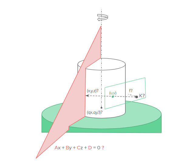
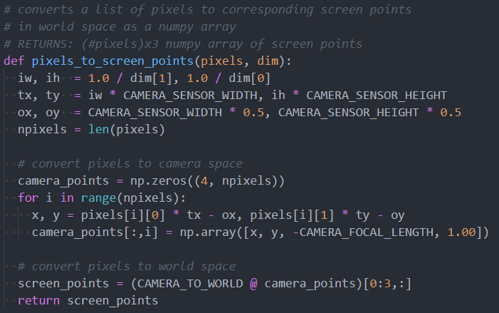
The method for transformation between pixel space and world space is given by the following equation:

λu=K(Rp+T)

Where K and λ are computed during intrinsic camera calibration, and R and T are computed during extrinsic camera calibration. We can then map the pixel where the center of the turntable is to a point in world space, q, with a fixed z=0, and a rotational direction of +z (relative to the camera perspective).

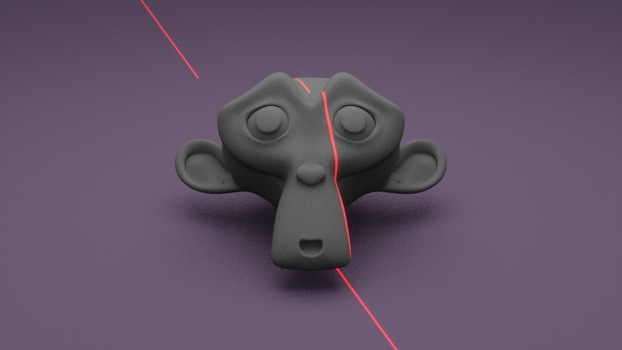
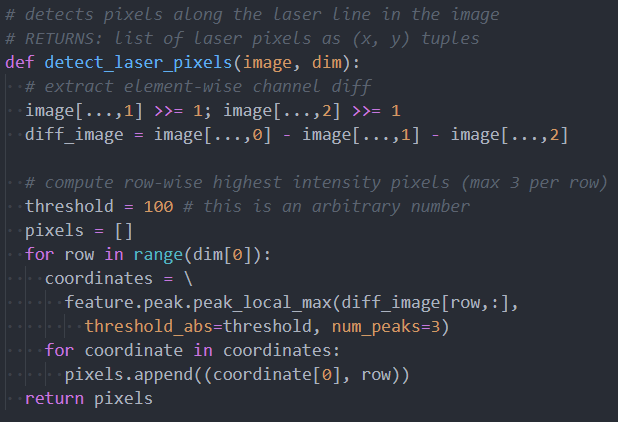
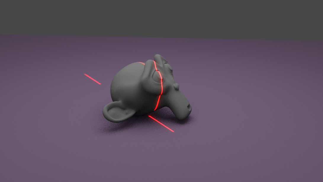
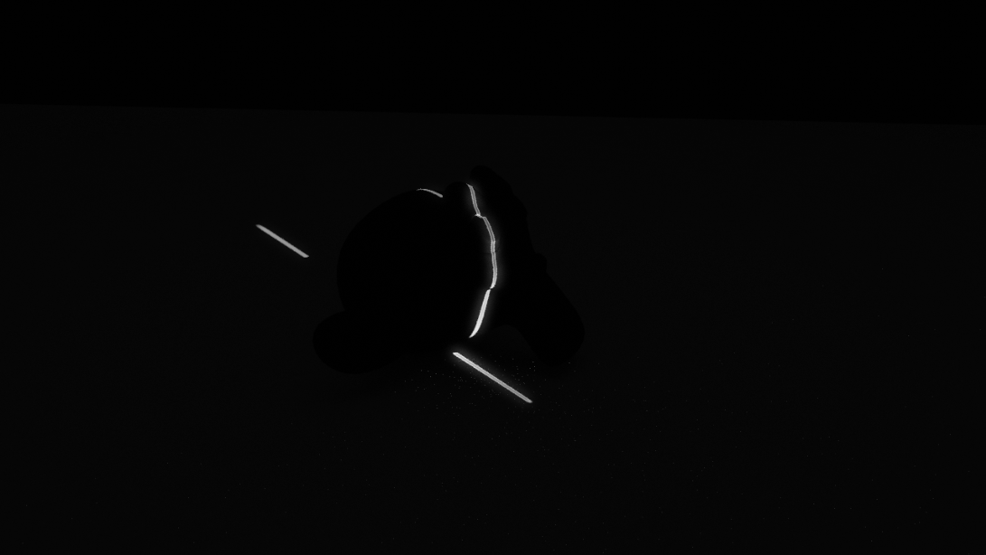
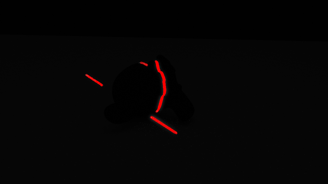
To calibrate the plane of the laser line, we first need image laser detection. We will compute this by first applying two filters to the image:

1. A filter that intensifies pixels with color similar to the laser’s light frequency
2. A horizontal gaussian filter

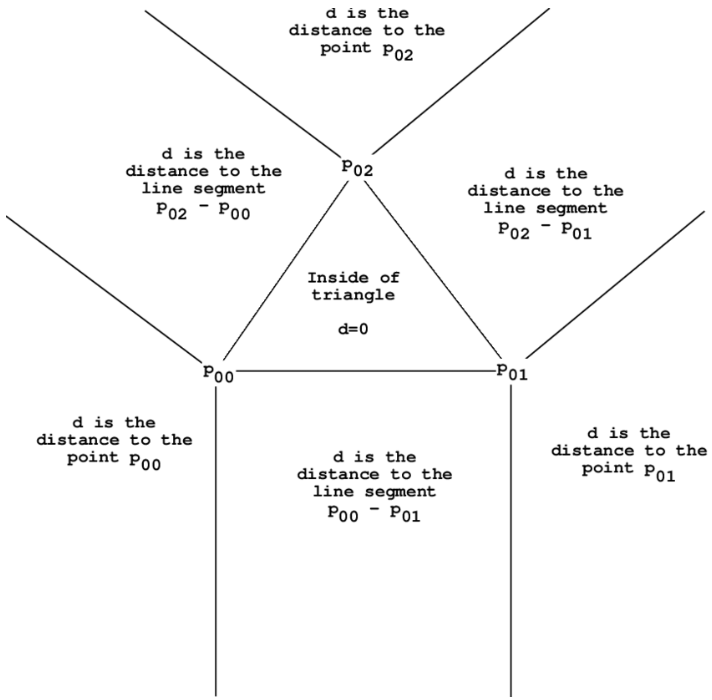
Then, for each row, we find the center of the gaussian distribution and that is the horizontal position of the laser line. If no intensity above a threshold is found, then that row does not contain the laser. Note that this solution prevents detection of multiple laser points within a single row, but this case will only occur with high surface curvature and can be resolved by our single-object multiple-scan procedure.

Laser plane calibration then happens by having a flat object on the turntable to allow for image laser detection. This allows us to find a set of points which are on the plane, which we can use to then solve a linear equation to compute the A, B, C, and D parameters of the plane of the laser line in world space. There is a slight caveat here. Since the laser itself is not changing angle or position, the points we capture do not identify a single plane, but rather a pencil of planes. To accommodate this, we will rotate the known calibration object (a checkerboard) to provide a set of non-collinear points. These points will allow us to solve the linear equation.

Calibration parameters will be solved for in the least-squared error sense, to match our recorded points. Global optimization will then be applied to all the parameters to reduce reconstruction error. Our implementation of optimization will probably consist of linear regression.

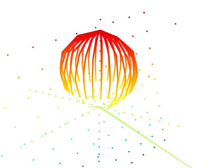
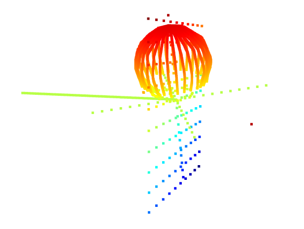
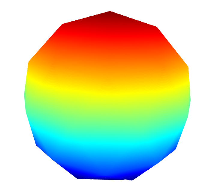
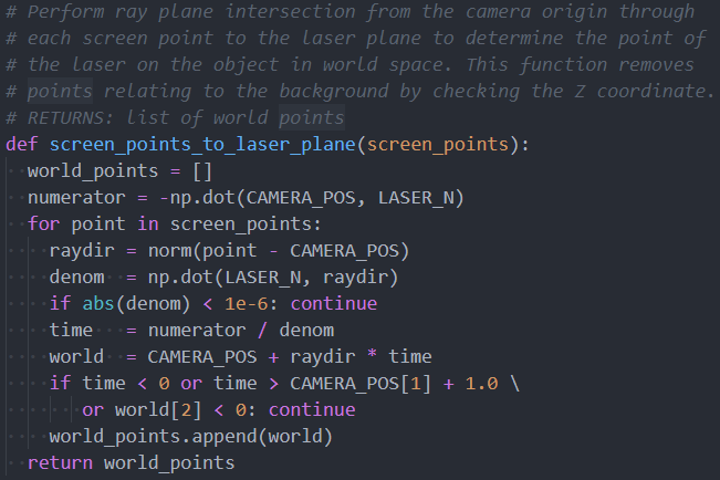
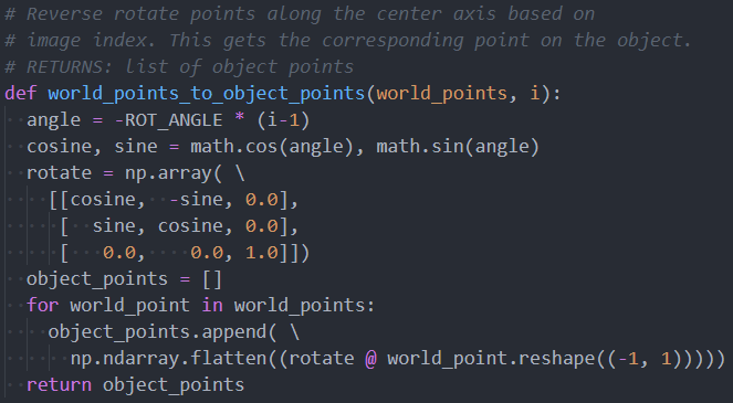
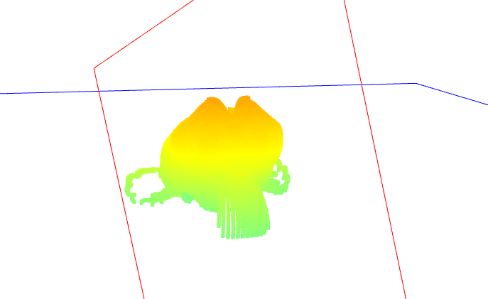
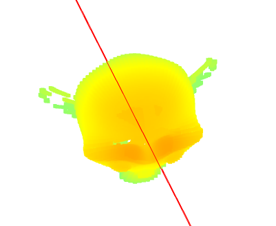
Once calibration is done, to generate 3D point cloud data we simply perform ray-plane intersection between the ray originating at the world space of the pixel with the laser line away from the camera position towards the laser plane in world space. This point is in world space coordinates, so it must be un-rotated around the rotational axis to get the corresponding point in object space. All such points are computed and aggregated together to form a point cloud. Multiple point clouds can then be combined using pairwise registration, which we will implement using the Iterative Closest Points (ICP) algorithm.

The ICP algorithm aims to compute the transformation between two point clouds by finding matching points between the point clouds. It is an iterative process that may converge on local minima, so it is important that multiple scans are not sufficiently far from each other in terms of angles.

Background points during 3D scanning can be removed if they fall under an intensity threshold in the laser-filtered image, and unrelated foreground points (such as points on the turntable) can be removed by filtering out points with a z coordinate of close to or less than 0.

Since we will not be getting our parts for a while, our next steps are to find ground truth models with which to test, and begin writing our verification code to test similarity between our mesh and the ground-truth. To avoid risk related to project schedule timing (and the lack of significant remaining time), I will be writing the initial prototyping code next week so that once the parts arrive we can begin early testing.