Jeremy’s Status Update for 05/03/2020

This week, I was mainly focusing on video editing. I worked on the bulk of our demo video and tried to make it high-production and professional with various 3D and text animations. It was quite a large amount of work (probably 30+ hours) to get this production quality but I think the result was quite good. We recorded all audio with Audacity and I used OBS Studio to create all the screen recordings, as well as Blender to create all the 3D animations. I used Premiere Pro to assemble everything and create cool text animations.

This is a screenshot of my Premiere Pro project.

This is a screenshot of the Blender project used to create the intro animation.

This is the Blender project for the intro shot with the sand blowing at the monkey. I used a more realistic and complex copper texture setup for the monkey and used Blender to simulate 15 million sand particles.

This is a screenshot of the Blender project used to recreate a realistic render of our original setup.

I tried to keep everything as close to the original as possible including our neoprene rubber over the plywood on the turntable, as well as setting up realistic textures for the camera and laser to look as close to the originals as possible.

Moving forward, I will be helping with the project report, the final deliverable for the Capstone class.

Jeremy’s Status Report for 04/26/2020

This week I mainly helped with the presentation and running a lot of tests to get good graphs for the slides. The slides can be found in the group slide deck, and I was mainly testing pixel skipping, laser threshold, and ICP number of point cloud inputs, and also did some testing on varying number of frames.

One key factor in development was time, as it took a lot of time to run any of these tests. From Saturday to Sunday when creating the slides I was basically rendering various number of frames such as 400, 700, and 1000, and also running the verification code on the side once one set of renders finished. Rendering is definitely the main bottle cap for the project in terms of how much time it takes to make changes, if the changes require re-rendering or rendering with new parameters.

I also fixed some bugs for ICP, with the main one being max iterations. Previously, our ICP was running max 30 iterations or until it converges, which I overlooked due to not printing the open3d inner debugging verbose output. However, from closer inspection, I realize that was causing a lot of the ICP outputs to not be nearly as perfectly aligned, and I set max iterations to 2000. For aligning point clouds, it usually takes between 40 to 150 iterations until convergence, and for our testing code to align meshes, it takes around 300 to 400 usually, so 2000 is a good upper cap which won’t restrict number of iterations a large majority of the time. Previously, ICP would have some random results and if we got lucky that the initial alignment was favorable then it would have better results, but now it actually converges on the local minima.

Next week I will be focusing on the demo videos and the final report.

Team Status Update for 04/19/2020

This week, our team focuses mainly on improving and making necessary fixes to our project. We also worked on preparing for the demo, by coming up with different test cases to show that we are achieving the requirements we have. We also discussed how to mimic issues that could potentially happen in the real world since we are using a simulation instead and will be working on that. We are also writing the testing code to compare the mesh we output and the ground truth mesh in order to output metrics that we can check against our accuracy requirements. 


Currently, there are no significant risks. 


There were no changes made to the existing design of our system. 


Below is the updated Gantt chart. 

https://docs.google.com/spreadsheets/d/1GGzn30sgRvBdlpad1TIZRK-Fq__RTBgIKN7kDVB3IlI/edit#gid=1867312600

Jeremy’s Status Update for 04/19/2020

This week, I focused on edge cases for ICP, some that Professor Tamal mentioned. There were three cases that I tested – scaling, z-translation, and misalignment in the scan. 


For scaling, I implemented a gradient descent-like algorithm that finds the correct scale factor. It uses the compute_pcd_distance function from open3d to get the average point to point distance between the two point clouds, then incrementally changes the scale factor by a specified delta until it reaches a local minima. There are still several issues with this approach as it assumes that the two point clouds are perfectly aligned; however, if the two point clouds have a scale error then the original ICP scan will align it somewhat well but not extremely well.

The results of the scaling algorithm is shown below, with “Result” referring to the result of local registration. I also tried testing to run the ICP pipeline again after determining the scale constant to better align the two point clouds, which should work in concept, but as of the time of writing this status report still has several bugs in it. You can tell from the ears that the source point cloud (orange) is smaller than the destination point cloud (blue). I simulated this in Blender by setting the object scale of the monkey to 0.7 for the orange, and 0.75 for the blue. This should give a scale factor of 1.07, but my algorithm outputs around 1.11 to 1.14 depending on a bit of the randomness of the ICP results, so there is still a bit of work to refine this part.

For z-translation, I simply moved the object upwards in Blender and performed the same scan. We can see that the orange point cloud is shifted below the blue. The results are near perfect as shown below.

For misalignment (x/y translation), I moved the monkey to be off center on the scan – see the animated gif for the pre-render setup. The monkey is now rotating off of its local center axis. 

Our scanning algorithm could handle this misalignment, and using ICP, I was able to re-align it with the original monkey, which worked basically the same as z-translation. We can see that the original point clouds simply has the orange point cloud shifted sideways.

Moving forward, I will refine the scaling algorithm and clean up the ICP pipeline, as well as assist in some of the testing code that Chakara and Alex is writing. The testing code also uses ICP to align the meshes before comparing them by converting the meshes to point clouds using an open3d sampling method, then getting the translation matrix from ICP and applying that to the original mesh.

Jeremy’s Status Update for 04/12/2020

This week I focused on the ICP algorithm as well as helping Alex with his code. One of our issues with the monkey was that its ears could not be scanned, so I started working on the ICP algorithm using open3d functions. We were still working on fixing the laser detection algorithm and other parts of the code that was broken this week, so I used some example point clouds to develop my code.

The ICP algorithm determines the transformation between two point clouds from different angles of the object by using least squares to match duplicate points – these point clouds would be constructed by mapping the scanned pixel and depth to their corresponding 3D cartesian coordinates as shown from the math above. Similar to gradient descent, ICP works best when starting at a good starting point to avoid being stuck at local minima and also save computation time.

Thus, there are actually two steps for ICP. The first step is called global registration, which uses downsampling with a voxel size in order to find an approximate transformation matrix to be fed into the local registration step. The global registration step can allow for any sort of transformations, and as an example, this is the starting point between the two meshes:

Next, the meshes are downsampled with a specified voxel size, which in this case is 5cm, but will be tuned for our use case later. Then, global registration will find a transformation matrix that is close to the real one which gives a good approximation in combining the meshes:

Next, there are two different types of ICP registration – point to point, and point to plane. Point to plane tends to produce more accurate results, and here is the result from point to plane ICP registration. Again, note that local registration requires a transformation matrix that is almost at the right place, that is why the previous step with global registration is important. Otherwise, the resulting transformation matrix will not move much at all. 

This is an example of when point to point registration is slightly off, where the resulting meshes are a bit separate vertically:

Next week I will work on refining the ICP algorithm as well as testing it on our go-to meshes like the monkey and the vase.

Jeremy’s Status Update for 04/04/2020

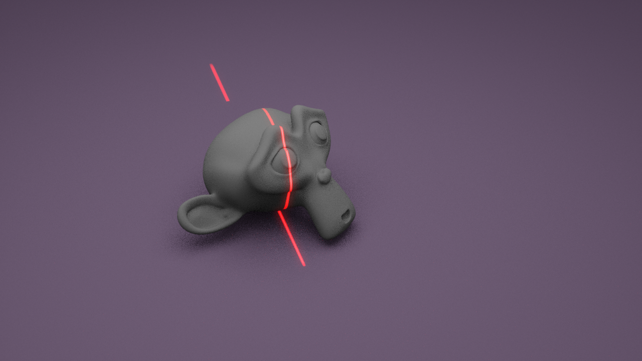
This week I finalized the simulation for the laser line camera input. I experimented with a few more objects and I also tuned the laser strength. Our laser line was previously too thick as shown below:

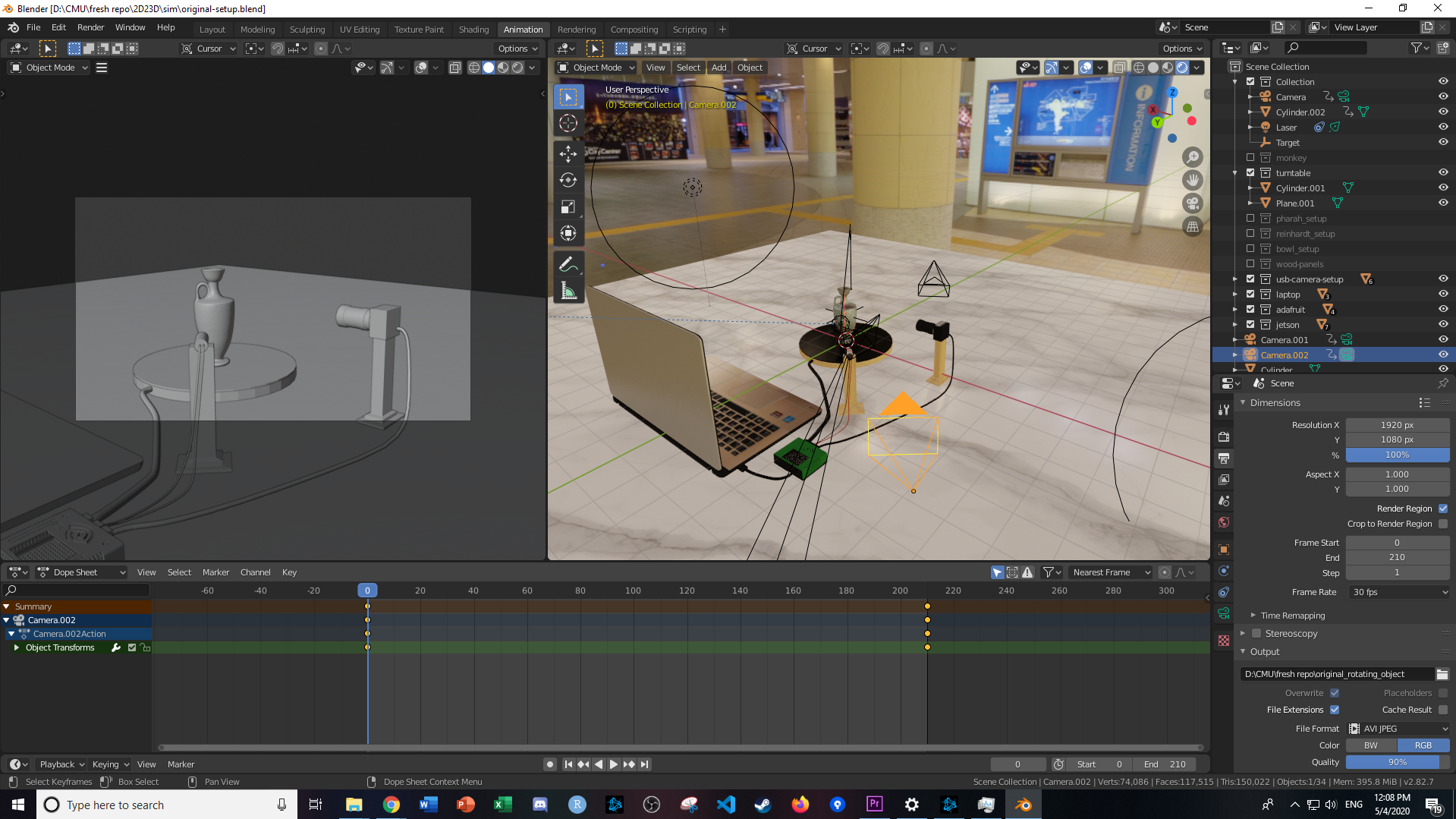
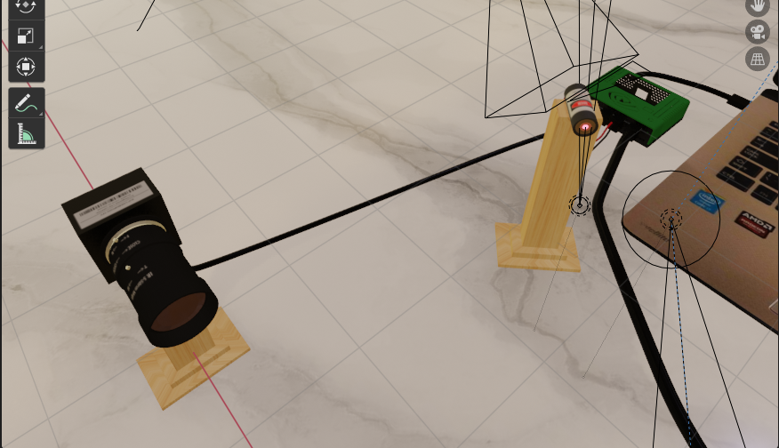
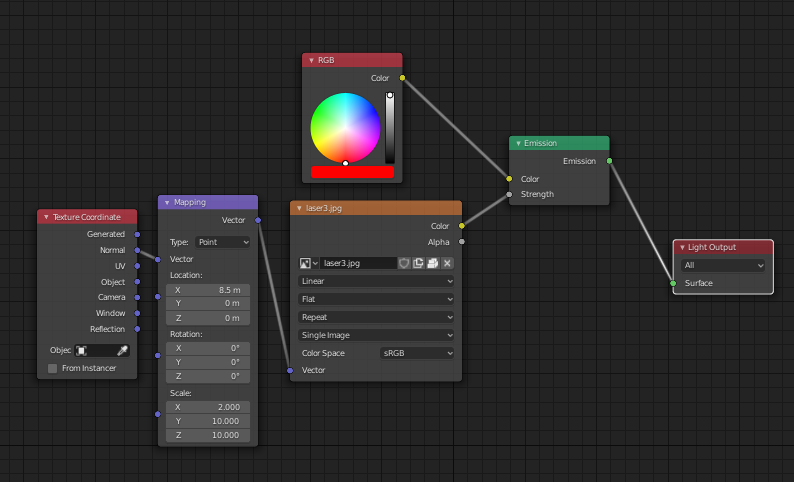
How the laser is currently being projected is that it is actually a light source projecting a black image with a thin white line in the middle added with a red tint. The current render setup is as follows:

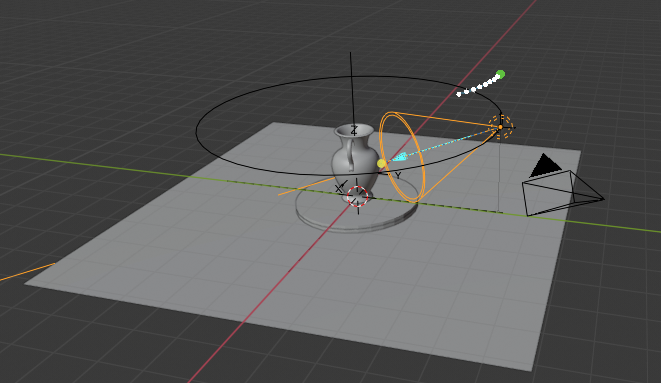
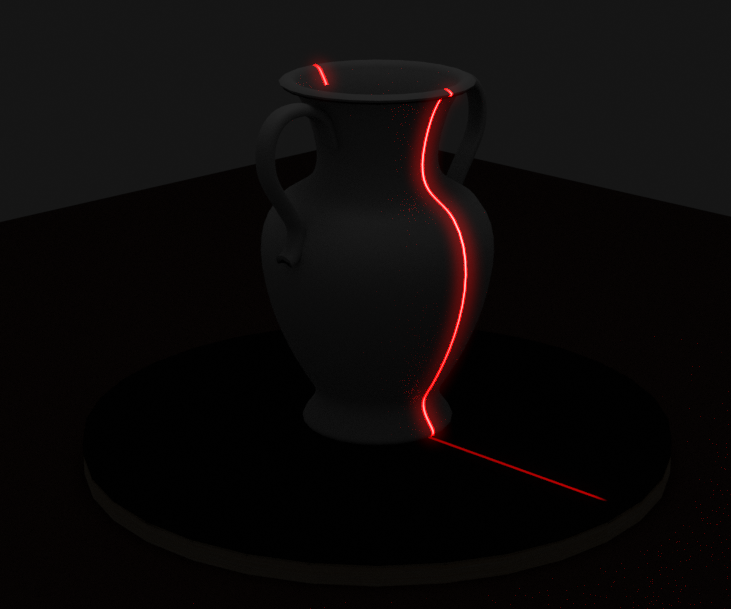
The orange selected cone is the laser projection source, and the object on the right with the triangle on top is the camera. The laser is currently at a height of 25 cm and I manually adjusted the laser to be able to cover the tallest allowed object which would be 30 cm tall. The camera is at a height of 40 cm and a 45 degree offset from the laser, at coordinates (70, 70, 40). The laser is at (0, 40, 25). After tuning the strength of the laser projection as well as the width, I obtained this render:

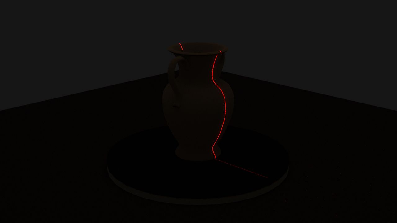
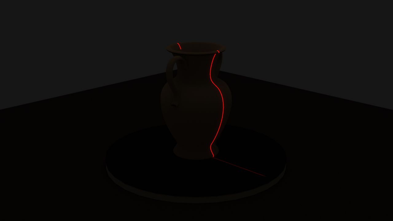
This was obtained at 32 samples meaning there are 32 samples per small box that Blender renders at a time (using Cycles Render). If we look closely (not sure how good the image will upload in WordPress) we can see some tiny red dots scattered around the image, and the laser line is also not crystal clear. This is due to Blender estimating some of the light bounces since we are sampling at such a low rate for the render. This can be fixed by bumping up the samples, as shown here with 512 samples.

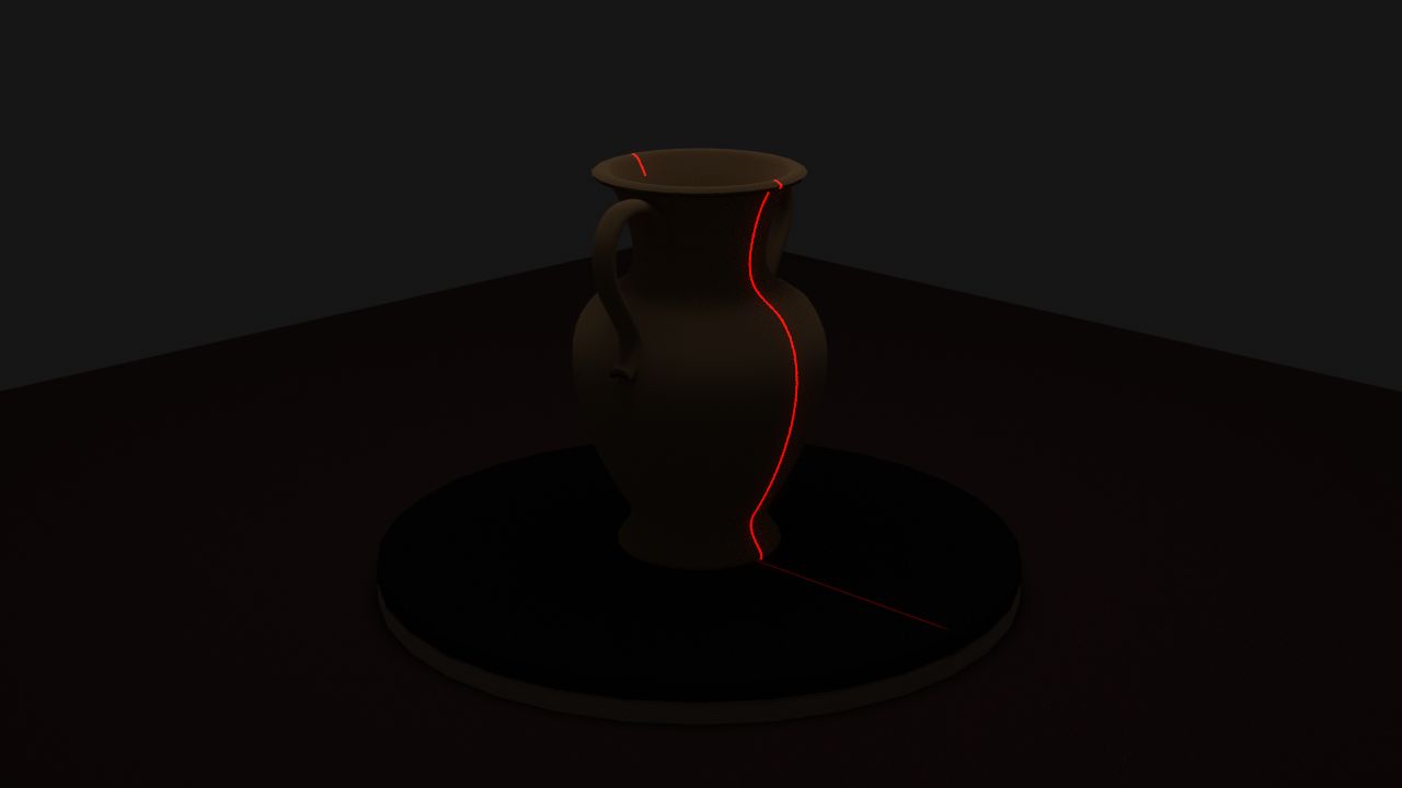
Our current light bounces is set to 1 to be realistic yet not cause too much diffuse in the render, and I can also control how much the laser glows. We can actually use a low sample rate to generate noise in a sense, and perhaps increase the number of light bounces to add more noise into the image. With 256 samples and 10 light bounces, we can start to see some red noise near the laser line (again I’m not sure how well images upload to WordPress):

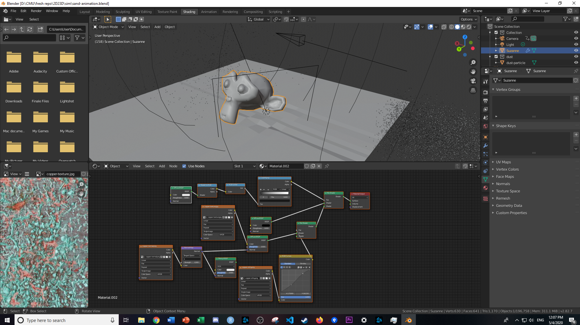
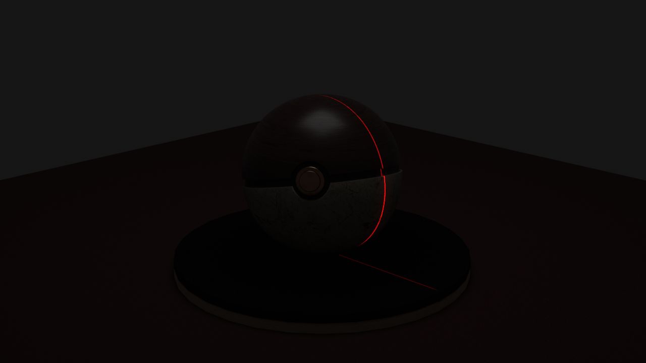
I also tried some other objects like this Pokeball but we will probably stick with the vase above for the in-lab demo.

One big cost is rendering time – especially with our original design where we would have 2000 frames, currently each frame with 32 samples only takes 8 seconds to render. This adds up to 16,000 seconds = 4.44 hours for 2000 frames. Thus, in terms of the user story, we will probably allow users to pre-select scanned images to demo. We will likely reduce the amount of frames as long as we can maintain a reasonable accuracy number. I was considering increasing sample rate and lowering the number of frames to get less noise per image, but I think keeping that noise in allows us to simulate what the real world image would’ve been like better. 

Our render resolution is 720p to simulate that of our original USB webcam. We will use 1 light bounce for our in-lab demo since we haven’t fully developed and tested our noise reduction for the images yet. 

Our current render parameters are:

Resolution 1280 x 720 (720p)
Samples 32
Light bounces 1 (initial development), 10+ (trying out noise reduction later)
Frames 30 (developing algos), 2000 (full test) – may likely change
Laser position (cm) (0, 40, 25)
Camera position (cm) (70, 70, 40)
Max object size (cm) 30 x 30 x 30
Render quality 80% (more realistic)
Laser intensity 50,000 W (a Blender specific parameter)
Laser blend 0.123 (how much it glows around the laser)

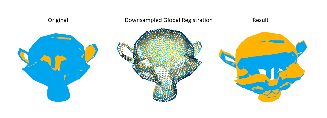
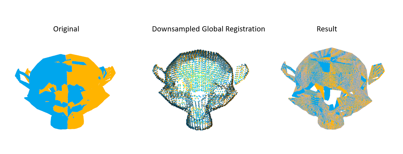
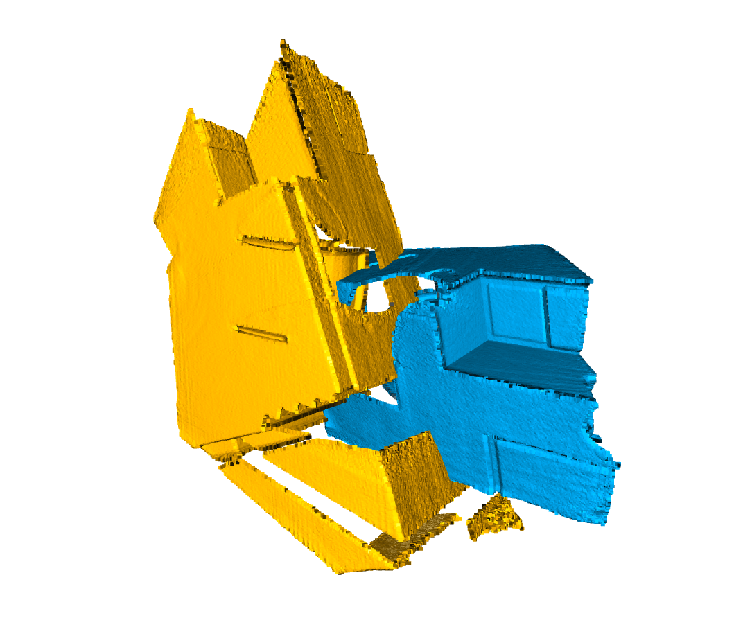
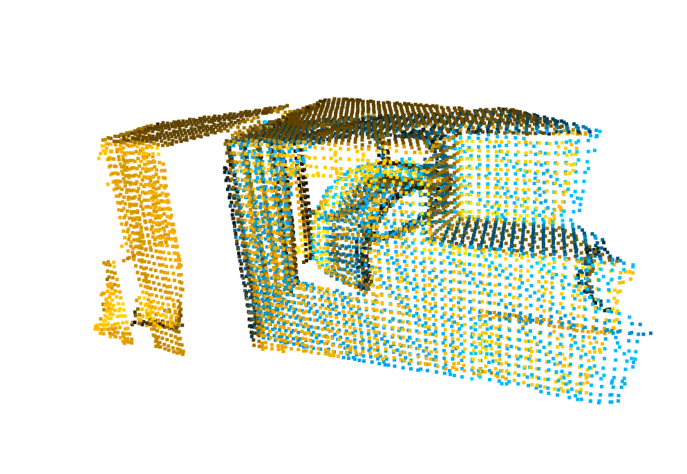
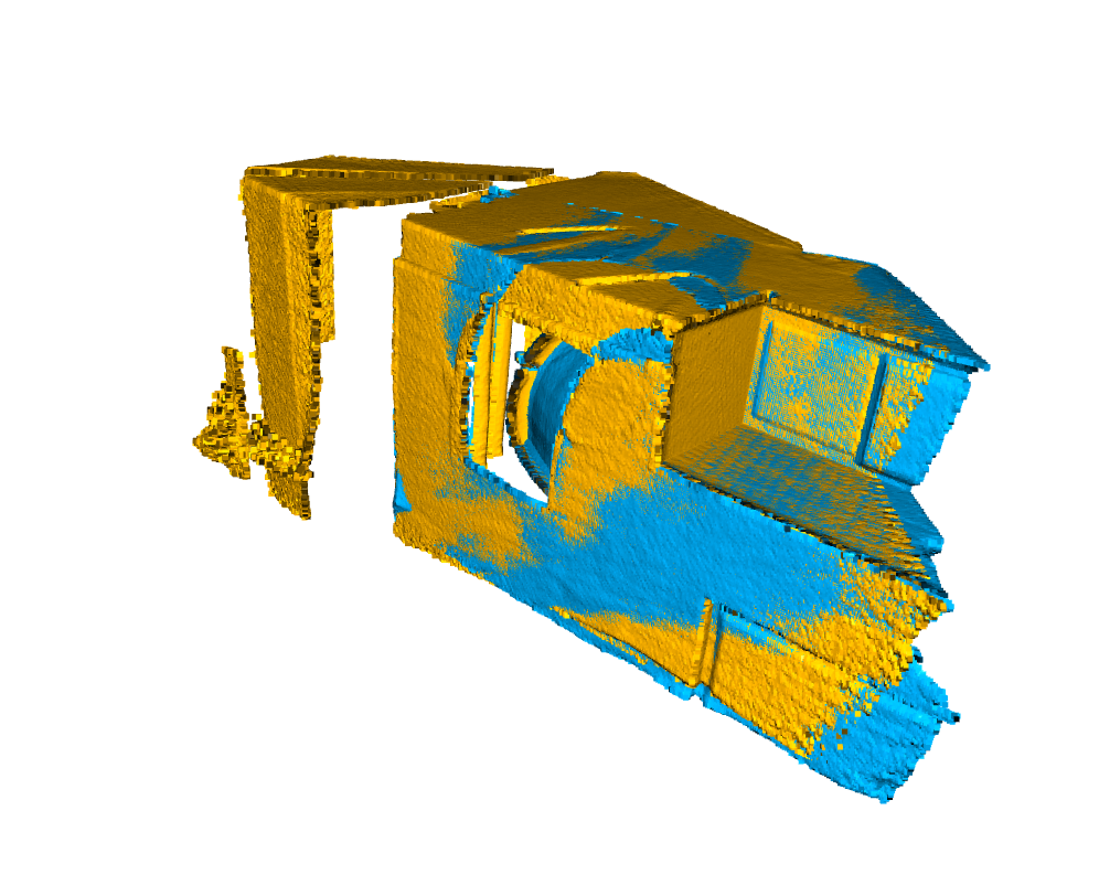
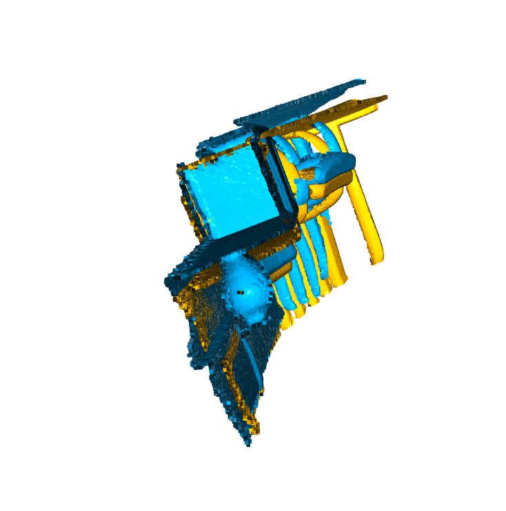
I will be helping the team finalize things for the demo the coming early week and start implementing ICP for combining scans as well after the demo.

Jeremy’s Status Update for 03/28/2020

This week I continued working on simulating the data we would get for the laser projection. I tweaked a few parameters and also got the animation to work. Now, Blender can either render a whole video or render a bunch of images with each frame of the video being saved as an image instead. We will use the set of images with a known rotation angle shift per image (360 degrees / number of frames) as input to our scanning software.

Here is the video of the rotating laser scan, where the laser is projecting from the right side: https://youtu.be/7rv-rFpyDcM

I updated the block diagram for our system – note that all the physical components have been removed, and the controllers are also removed. We have Blender-simulated data instead for the input, and we will likely use a Django web app for ease of running Python with a simple web interface rather than using some Python GUI like Tkinter which would take more unnecessary time to implement. Chakara and I are both experienced in developing web applications so using Django is more of a choice of saving time in a portion that isn’t entirely essential to the project. 

Moving forward, I will finalize the laser scan by adding a platform and also calibrating the angle between the camera and the laser, as well as the height of these two items. I will also start finding more objects that fit our project, and will look to start implementing some of the code to perform outlier removal on the point cloud.

Jeremy’s Status Update for 03/21/2020

As mentioned in the team status update, we are switching our project to simulate or generate images that we would normally get from the camera and laser setup instead of building a physical piece of hardware. I started to explore options to do this, and I will be using Blender modeling software to generate these images. In these few days, I successfully projected a laser stripe onto the default Blender object Susanne the monkey. 


This is a sample of the laser stripe projected onto the object. I will add a cylindrical platform with a wood texture and tune the background to be dark grey or something so we can see the laser better. 


This is the shading setup I used for the laser projection. I used an image with a white line of a few pixels wide down the middle and actually projected the image shaded with a red tint to resemble a laser stripe. I can tune how white or red the laser stripe is with the power parameter in Blender (set to 70,000W in the render above). I can also control how much red diffuses from the laser by tuning how many light bounces there will be in the render. 


Moving forward, I will be using keyframe animations to rotate an object around the z-axis and generate images resembling what we would get in our physical setup. I will need to first acquire our old materials from Quinn so I can assemble a basic non-moving version of our previous design to check how well my simulated images resemble it, and also get the camera parameters of our USB camera to calibrate those in Blender.

Team Status Update for 03/07/2020

This week, our team received the mechanical parts and started testing a few of the components. Currently, our risk is similar to last week’s which is mainly the motor and jetson integration, but we already talked to Professor Nace and we could check if Quinn has an extra Arduino. Thus, this risk is mitigated. Our parts also came in time and most of them worked as we expected. There were no changes being made to the existing design of the system yet.


This is the link to our updated schedule: https://docs.google.com/spreadsheets/d/1GGzn30sgRvBdlpad1TIZRK-Fq__RTBgIKN7kDVB3IlI/edit?usp=sharing

Jeremy’s Status Update for 03/07/2020

This week I assisted Chakara for the mechanical components of the rotating platform. I helped pick up components of our platform setup and test that they work. Chakara has included a table of the list of parts for his status report so I will avoid repeating that information here. I tested the laser strip diode and it seemed to work with an input voltage between 3 to 5 volts. The laser strip seems to be a bit wider at closer ranges so we will have to put the laser at a good enough distance for the strip to still be bright but not to be so wide as to mess up our laser detection algorithm. The camera also seems to be of a good resolution when we tested it with Facetime on Chakara’s Macbook, and should be good enough for our project. If not, we have a bit under $200 for getting a better camera or laser if needed.


For the mechanical subsystem of our device (see the design report), we will require significant physical pieces to build both the frame, motor components, and holders of the camera and laser line. This week we have gotten access to a bin to store our physical components as we work on them (bin #17). We have also attended the Tech Spark session to prepare us for laser cutting (for a sheet gear) and 3D printing (for the axis gear). If we find that these gears wear down over usage, we may need to allocate an additional part of our remaining budget to buy metal gears.


I also looked into the gear components and will be looking to create the files necessary to laser cut our acrylic piece as well as create the gear piece to fit onto the stepper motor. Throughout spring break, I will be out of town and will not work extensively on the project, as planned in the Gantt chart. However, I will still aim to create the files for the gear piece and the acrylic. I will also start to assemble our testing database by finding free 3D models online that fit our requirements. After break, I will start writing code for the triangulation step as well as ICP and pairwise registration as described in our design report and presentation.