Category: Uncategorized

This week I mainly helped with the presentation and running a lot of tests to get good graphs for the slides. The slides can be found in the group slide deck, and I was mainly testing pixel skipping, laser threshold, and ICP number of point cloud inputs, and also did some testing on varying number of frames.

One key factor in development was time, as it took a lot of time to run any of these tests. From Saturday to Sunday when creating the slides I was basically rendering various number of frames such as 400, 700, and 1000, and also running the verification code on the side once one set of renders finished. Rendering is definitely the main bottle cap for the project in terms of how much time it takes to make changes, if the changes require re-rendering or rendering with new parameters.

I also fixed some bugs for ICP, with the main one being max iterations. Previously, our ICP was running max 30 iterations or until it converges, which I overlooked due to not printing the open3d inner debugging verbose output. However, from closer inspection, I realize that was causing a lot of the ICP outputs to not be nearly as perfectly aligned, and I set max iterations to 2000. For aligning point clouds, it usually takes between 40 to 150 iterations until convergence, and for our testing code to align meshes, it takes around 300 to 400 usually, so 2000 is a good upper cap which won’t restrict number of iterations a large majority of the time. Previously, ICP would have some random results and if we got lucky that the initial alignment was favorable then it would have better results, but now it actually converges on the local minima.

Next week I will be focusing on the demo videos and the final report.

This week I focused on the ICP algorithm as well as helping Alex with his code. One of our issues with the monkey was that its ears could not be scanned, so I started working on the ICP algorithm using open3d functions. We were still working on fixing the laser detection algorithm and other parts of the code that was broken this week, so I used some example point clouds to develop my code.

The ICP algorithm determines the transformation between two point clouds from different angles of the object by using least squares to match duplicate points – these point clouds would be constructed by mapping the scanned pixel and depth to their corresponding 3D cartesian coordinates as shown from the math above. Similar to gradient descent, ICP works best when starting at a good starting point to avoid being stuck at local minima and also save computation time.

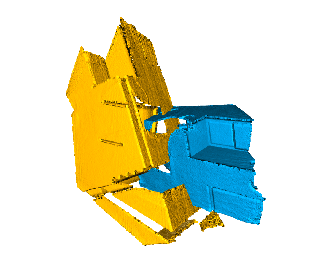
Thus, there are actually two steps for ICP. The first step is called global registration, which uses downsampling with a voxel size in order to find an approximate transformation matrix to be fed into the local registration step. The global registration step can allow for any sort of transformations, and as an example, this is the starting point between the two meshes:

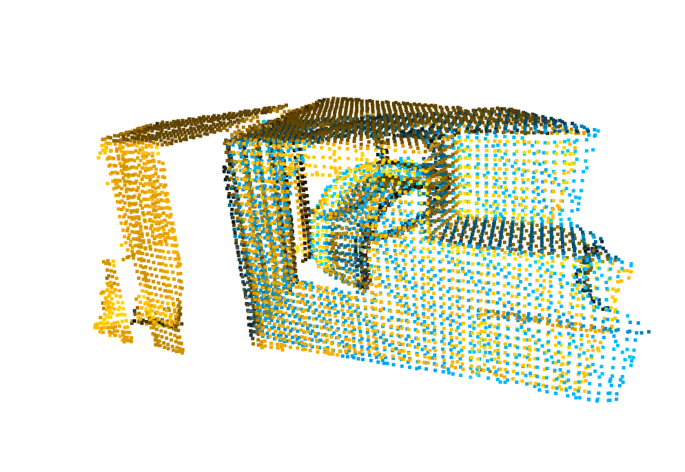
Next, the meshes are downsampled with a specified voxel size, which in this case is 5cm, but will be tuned for our use case later. Then, global registration will find a transformation matrix that is close to the real one which gives a good approximation in combining the meshes:

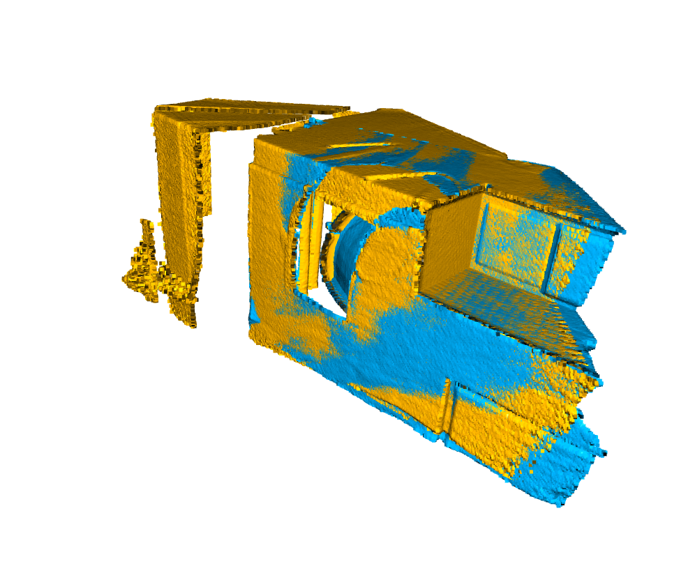
Next, there are two different types of ICP registration – point to point, and point to plane. Point to plane tends to produce more accurate results, and here is the result from point to plane ICP registration. Again, note that local registration requires a transformation matrix that is almost at the right place, that is why the previous step with global registration is important. Otherwise, the resulting transformation matrix will not move much at all. 

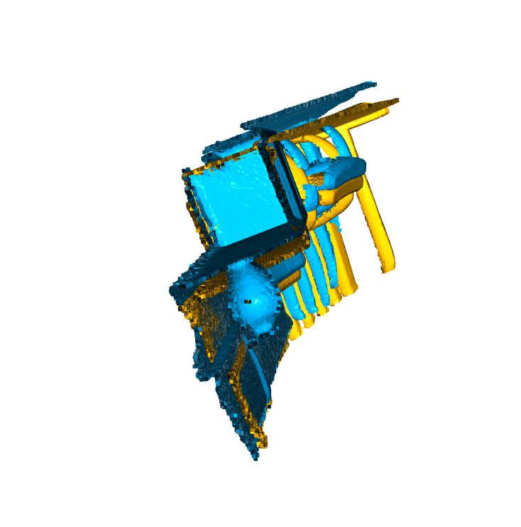
This is an example of when point to point registration is slightly off, where the resulting meshes are a bit separate vertically:

Next week I will work on refining the ICP algorithm as well as testing it on our go-to meshes like the monkey and the vase.

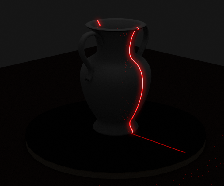
This week I finalized the simulation for the laser line camera input. I experimented with a few more objects and I also tuned the laser strength. Our laser line was previously too thick as shown below:

How the laser is currently being projected is that it is actually a light source projecting a black image with a thin white line in the middle added with a red tint. The current render setup is as follows:

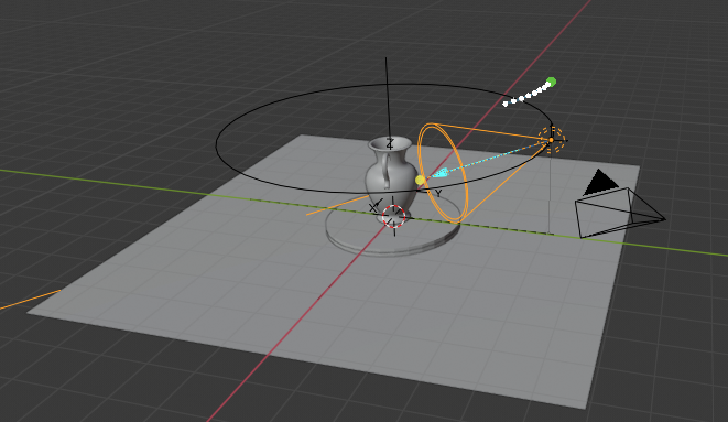
The orange selected cone is the laser projection source, and the object on the right with the triangle on top is the camera. The laser is currently at a height of 25 cm and I manually adjusted the laser to be able to cover the tallest allowed object which would be 30 cm tall. The camera is at a height of 40 cm and a 45 degree offset from the laser, at coordinates (70, 70, 40). The laser is at (0, 40, 25). After tuning the strength of the laser projection as well as the width, I obtained this render:

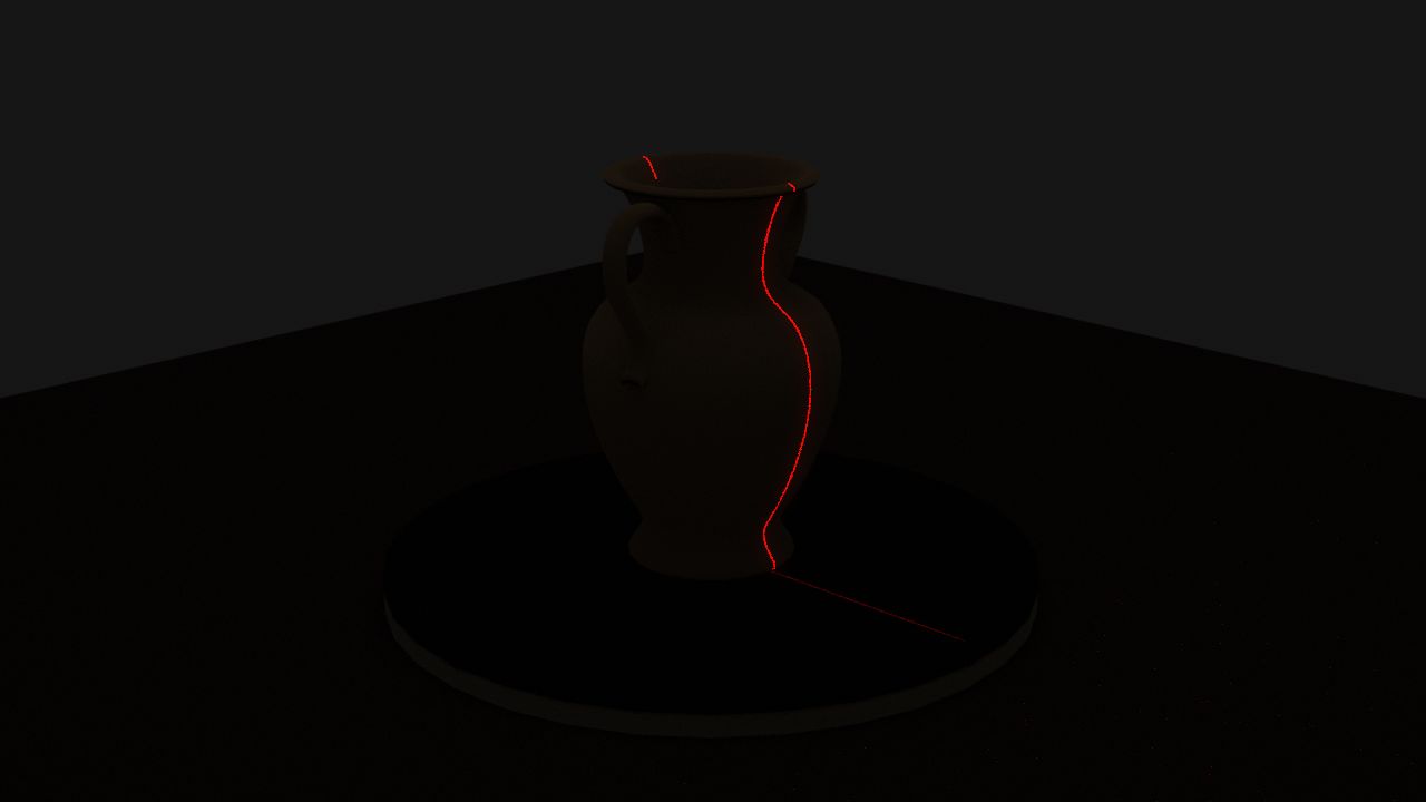
This was obtained at 32 samples meaning there are 32 samples per small box that Blender renders at a time (using Cycles Render). If we look closely (not sure how good the image will upload in WordPress) we can see some tiny red dots scattered around the image, and the laser line is also not crystal clear. This is due to Blender estimating some of the light bounces since we are sampling at such a low rate for the render. This can be fixed by bumping up the samples, as shown here with 512 samples.

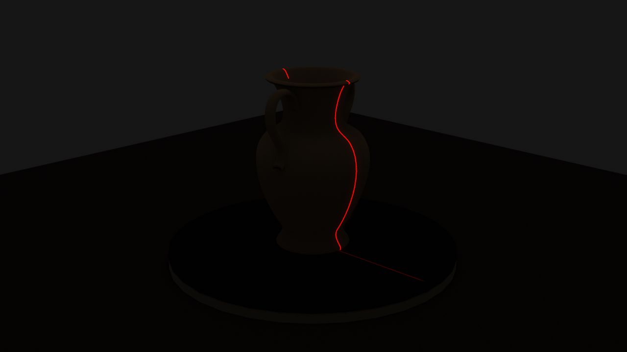
Our current light bounces is set to 1 to be realistic yet not cause too much diffuse in the render, and I can also control how much the laser glows. We can actually use a low sample rate to generate noise in a sense, and perhaps increase the number of light bounces to add more noise into the image. With 256 samples and 10 light bounces, we can start to see some red noise near the laser line (again I’m not sure how well images upload to WordPress):

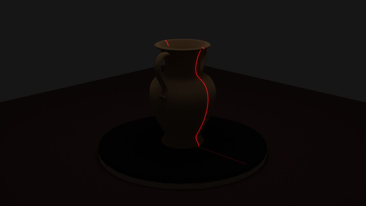
I also tried some other objects like this Pokeball but we will probably stick with the vase above for the in-lab demo.

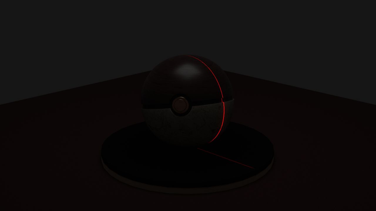
One big cost is rendering time – especially with our original design where we would have 2000 frames, currently each frame with 32 samples only takes 8 seconds to render. This adds up to 16,000 seconds = 4.44 hours for 2000 frames. Thus, in terms of the user story, we will probably allow users to pre-select scanned images to demo. We will likely reduce the amount of frames as long as we can maintain a reasonable accuracy number. I was considering increasing sample rate and lowering the number of frames to get less noise per image, but I think keeping that noise in allows us to simulate what the real world image would’ve been like better. 

Our render resolution is 720p to simulate that of our original USB webcam. We will use 1 light bounce for our in-lab demo since we haven’t fully developed and tested our noise reduction for the images yet. 

Our current render parameters are:

Resolution	1280 x 720 (720p)
Samples	32
Light bounces	1 (initial development), 10+ (trying out noise reduction later)
Frames	30 (developing algos), 2000 (full test) – may likely change
Laser position (cm)	(0, 40, 25)
Camera position (cm)	(70, 70, 40)
Max object size (cm)	30 x 30 x 30
Render quality	80% (more realistic)
Laser intensity	50,000 W (a Blender specific parameter)
Laser blend	0.123 (how much it glows around the laser)

I will be helping the team finalize things for the demo the coming early week and start implementing ICP for combining scans as well after the demo.