Chakara’s Status Update for 04/19/2020

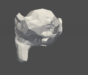
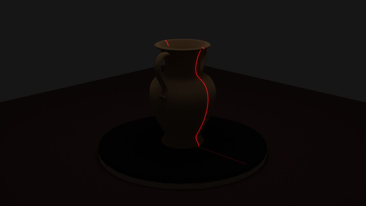
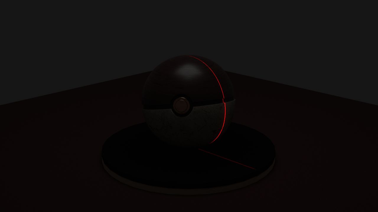
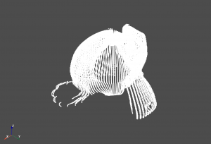
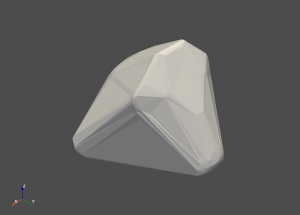
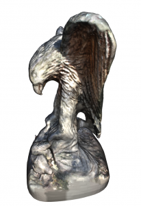
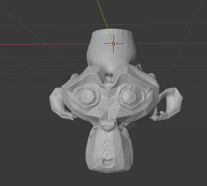
This week, on top of working with other team members on preparing for the in-lab demo and thinking of different testing we could perform, I mainly worked on improving the triangulation algorithm. As mentioned in last week’s report, the triangulated meshes using different algorithms were not satisfiable. The Screened Poisson Reconstruction proposed in Kazhdan and Hoppe’s paper looked the most promising; thus I decided to try fixing it. 


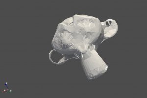
I first tried working on other example pcd files from the web, and the Poisson Reconstruction algorithm worked perfectly. 

I looked deeper into the pcd files and the only two main differences were just that example pcd files also contain FIELDS normal_x, normal_y, and normal_z which have normals information. Thus, my speculation was correct. 


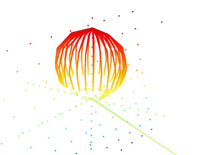
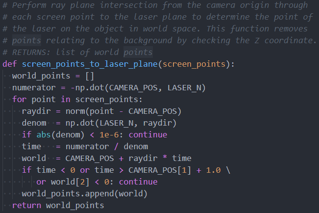
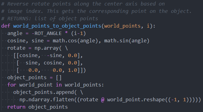
I then tried orienting the normals to align with the direction of the camera position and laser position but they still didn’t work. 


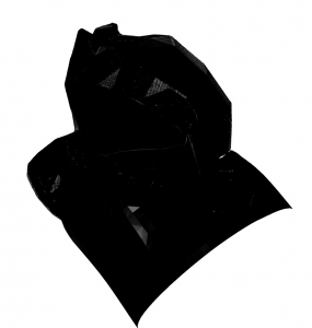
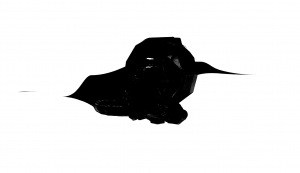
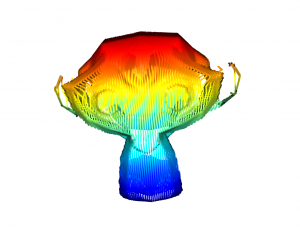
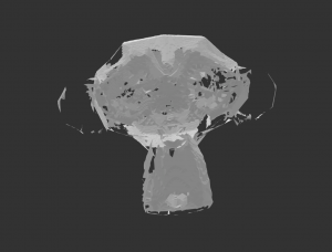
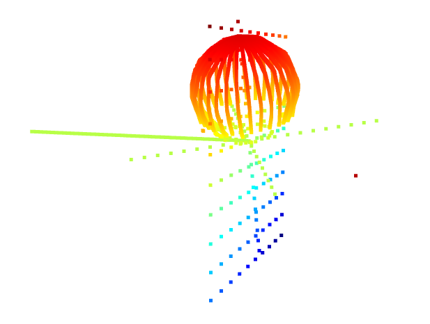
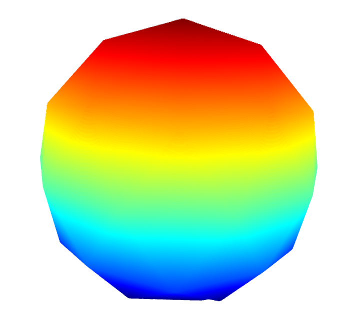
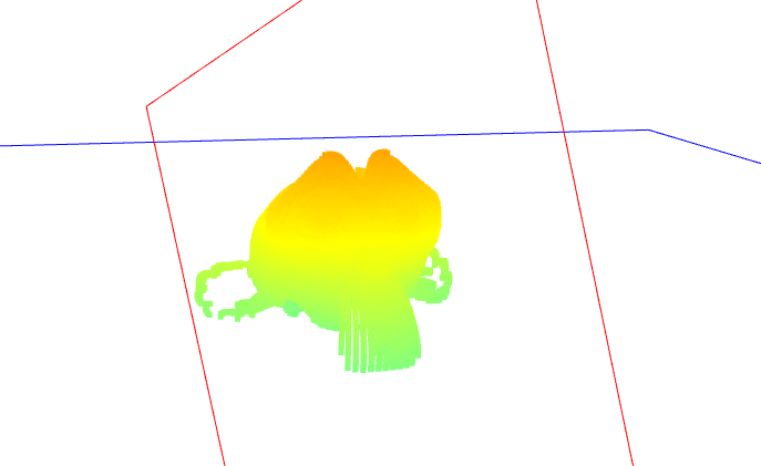
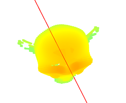
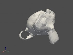
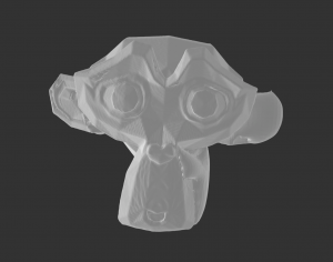
After that, I tried adjusting the search parameter when estimating the normals. I changed from the default search tree to o3d.geometry.KDTreeSearchParamHybrid which I can adjust the number of neighbors and the radius size to look at when estimating the normals for each point in the point cloud. After estimating the normals, I then orient the normals such that the normals are all pointing inward and invert the normals out so that all the normals are pointing directly outward from the surface. The results are much more promising. The smoothed results were not as accurate so I decided to ignore smoothing. 

I then realigned the normals to get rid of the weird vase shape by making sure that the z-axis alignment of the normals was at the center of the point cloud. 

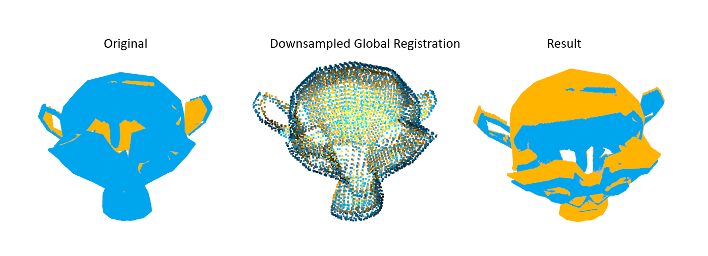
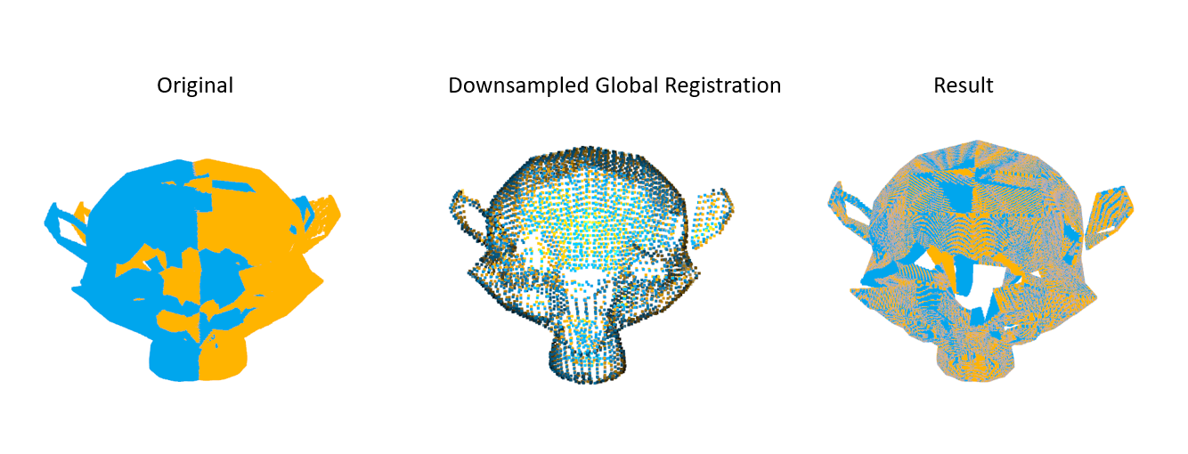
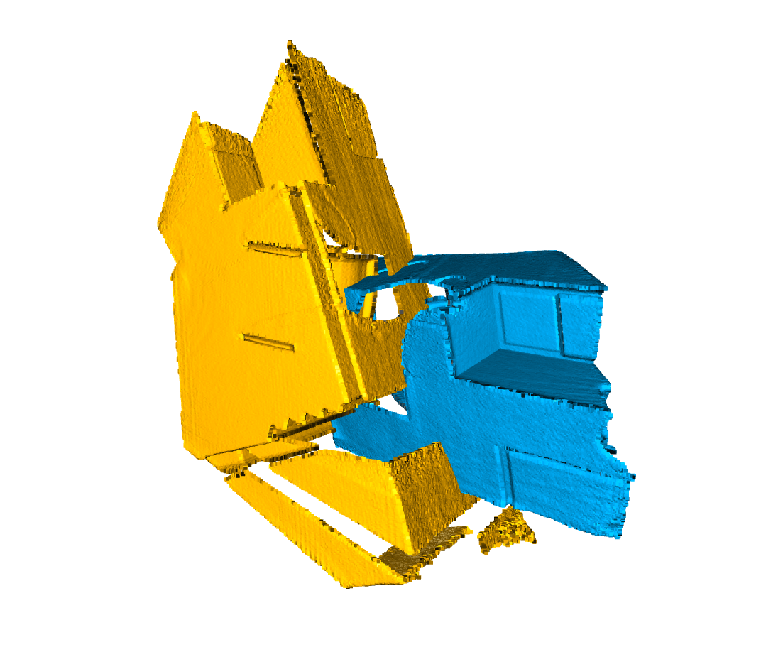
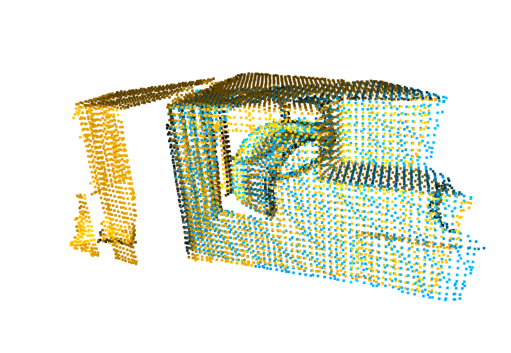
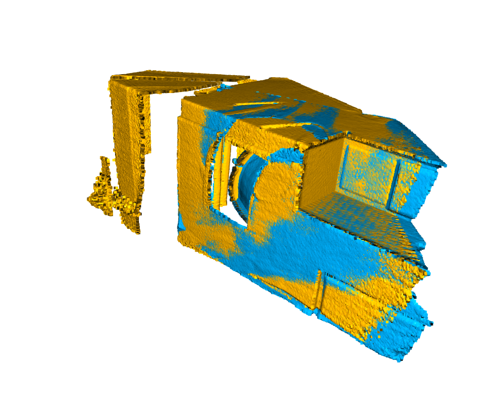
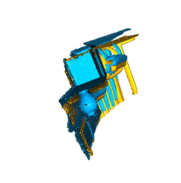
After that, I helped Alex work on the verification by writing a function to get the accuracy percentage. I used Alex’s work on getting the distances between the target and the source and wrote a simple function to check if 90% of the points are within 5% of the longest axis and 100% of the points are within 2% of the longest axis. 

I am currently on schedule. For next week, I hope to fully finish verification and help the team prepare for the final presentation and demo videos. 

Jeremy’s Status Update for 04/19/2020

This week, I focused on edge cases for ICP, some that Professor Tamal mentioned. There were three cases that I tested – scaling, z-translation, and misalignment in the scan. 


For scaling, I implemented a gradient descent-like algorithm that finds the correct scale factor. It uses the compute_pcd_distance function from open3d to get the average point to point distance between the two point clouds, then incrementally changes the scale factor by a specified delta until it reaches a local minima. There are still several issues with this approach as it assumes that the two point clouds are perfectly aligned; however, if the two point clouds have a scale error then the original ICP scan will align it somewhat well but not extremely well.

The results of the scaling algorithm is shown below, with “Result” referring to the result of local registration. I also tried testing to run the ICP pipeline again after determining the scale constant to better align the two point clouds, which should work in concept, but as of the time of writing this status report still has several bugs in it. You can tell from the ears that the source point cloud (orange) is smaller than the destination point cloud (blue). I simulated this in Blender by setting the object scale of the monkey to 0.7 for the orange, and 0.75 for the blue. This should give a scale factor of 1.07, but my algorithm outputs around 1.11 to 1.14 depending on a bit of the randomness of the ICP results, so there is still a bit of work to refine this part.

For z-translation, I simply moved the object upwards in Blender and performed the same scan. We can see that the orange point cloud is shifted below the blue. The results are near perfect as shown below.

For misalignment (x/y translation), I moved the monkey to be off center on the scan – see the animated gif for the pre-render setup. The monkey is now rotating off of its local center axis. 

Our scanning algorithm could handle this misalignment, and using ICP, I was able to re-align it with the original monkey, which worked basically the same as z-translation. We can see that the original point clouds simply has the orange point cloud shifted sideways.

Moving forward, I will refine the scaling algorithm and clean up the ICP pipeline, as well as assist in some of the testing code that Chakara and Alex is writing. The testing code also uses ICP to align the meshes before comparing them by converting the meshes to point clouds using an open3d sampling method, then getting the translation matrix from ICP and applying that to the original mesh.

Chakara’s Status Update for 04/11/2020

This week, after Alex made fixes to the point cloud construction algorithm, I tried testing the new pcd files on our current triangulation algorithm. The rendered object looks perfect.

However, testing a more complicated object such as a monkey, the triangle meshes look a little rough and might not meet our accuracy requirements. 

I looked into the point cloud and it is very detailed so the problem is with the delaunay technique we are currently using. Although I tried changing different parameters, the results are still not satisfiable. 

Thus, I started looking into other libraries which might have other techniques. I ended up trying open3d this week. The first technique I try is to compute a convex hull of the point cloud and generate a mesh from that, the result is very not satisfiable since the convex hull is just a set of points is defined as the smallest convex polygon, that encloses all of the points in the set. Thus, it only creates an outer rough polygon surface of the monkey. 

After that, I tried the pivoting ball technique. This implements the Ball Pivoting algorithm proposed in F. Bernardini et al. The surface reconstruction is done by rolling a ball with a given radius over the point cloud, whenever the ball touches three points a triangle is created, and I could adjust the radii of the ball that are used for the surface reconstruction. I computed the radii by finding the norms of all the closest distance between every point in the point cloud and multiply it by a constant. Using a constant smaller than 5, the results were not satisfiable. The results got more accurate as I increased the constant size; however, a constant above 15 takes longer than 5 minutes to compute using my computer which would not pass our efficiency requirement, and the results were still not as satisfiable as I hoped for. I tried different smoothing techniques but they did not help much. 

The next technique I used was the poisson technique. This implements the Screened Poisson Reconstruction proposed in Kazhdan and Hoppe. From this method, I can vary the depth, width, scale, and the linear fit of the algorithm. The depth is the maximum depth of the tree that will be used for surface reconstruction. The width specifies the target width of the finest level octree cells. The scale specifies the ratio between the diameter of the cube used for reconstruction and the diameter of the samples’ bounding cube. And linear fit can tell if the reconstructor uses linear interpolation to estimate the positions of iso-vertices or not. 

The results are accurate and look smooth once I normalize the normals but there is a weird surface. By looking at the pcd file and a voxel grid (below), there are no points where this weird rectangular surface lies. 

Currently, I assumed that the weird surface is from the directions the normals are oriented to, since the location of the surface changes when I orient the normals differently.

I’m currently a little behind schedule since I hoped to fully finish triangulation, but luckily, our team allocated enough slack time for me to fix this. If I finish early, I hope to help the team work on the testing benchmarks and adding noise.  

For next week, I hope to be able to fix this issue, either by applying different other techniques on top of the poisson technique or changing to marching cubes algorithm which also seems probable.

Team Status Update for 04/11/2020

This week, our team focuses mainly on fixing accuracy issues with the laser detection, point cloud construction, and triangulation algorithms. Most of our work was done separately. For next week, we plan on preparing for the demo, finish adding noises and writing testing benchmarks, and making any necessary final fixes.

Currently, there are no significant risks. 

There were no changes made to the existing design of our system. 

Below is the updated Gantt chart. 

https://docs.google.com/spreadsheets/d/1GGzn30sgRvBdlpad1TIZRK-Fq__RTBgIKN7kDVB3IlI/edit#gid=1867312600

Jeremy’s Status Update for 04/12/2020

This week I focused on the ICP algorithm as well as helping Alex with his code. One of our issues with the monkey was that its ears could not be scanned, so I started working on the ICP algorithm using open3d functions. We were still working on fixing the laser detection algorithm and other parts of the code that was broken this week, so I used some example point clouds to develop my code.

The ICP algorithm determines the transformation between two point clouds from different angles of the object by using least squares to match duplicate points – these point clouds would be constructed by mapping the scanned pixel and depth to their corresponding 3D cartesian coordinates as shown from the math above. Similar to gradient descent, ICP works best when starting at a good starting point to avoid being stuck at local minima and also save computation time.

Thus, there are actually two steps for ICP. The first step is called global registration, which uses downsampling with a voxel size in order to find an approximate transformation matrix to be fed into the local registration step. The global registration step can allow for any sort of transformations, and as an example, this is the starting point between the two meshes:

Next, the meshes are downsampled with a specified voxel size, which in this case is 5cm, but will be tuned for our use case later. Then, global registration will find a transformation matrix that is close to the real one which gives a good approximation in combining the meshes:

Next, there are two different types of ICP registration – point to point, and point to plane. Point to plane tends to produce more accurate results, and here is the result from point to plane ICP registration. Again, note that local registration requires a transformation matrix that is almost at the right place, that is why the previous step with global registration is important. Otherwise, the resulting transformation matrix will not move much at all. 

This is an example of when point to point registration is slightly off, where the resulting meshes are a bit separate vertically:

Next week I will work on refining the ICP algorithm as well as testing it on our go-to meshes like the monkey and the vase.

Alex’s Status Update for 04/11/2020

This week I fixed all the bugs (that I could find) which appeared during our team’s demo on Monday. The main two issues we were facing from surface-level inspection were seemingly large amounts of outlier points remaining in the final point cloud, and overall geometric distortion of the point cloud. For example, the iteration of our code that was ready for the Monday demo seemed to have two top layers to the scan of the cube, even though it should be one flat surface.

After further inspection of our code to generate the point cloud and significant research into similar applications such as path tracing to perform realistic lighting simulations (both path tracing and laser triangulation require ray-scene intersection algorithms, in which the slightest incorrect implementation can cause unrecognizable visual outputs), I realized some of the problems were a result of me making small errors that propagated to have a hugely unreliable output.

To explain the cause of the bugs, I will first re-introduce the problem in a fresh light to see where we went wrong in our first attempt. To reiterate, the core of the laser triangulation algorithm is finding the “depth” of each pixel along the laser line in an image. Once we have this depth, we can compute the 3D coordinate of the laser point by travelling towards that pixel’s direction into the scene by the depth. This depth can be computed by shooting a ray from the origin of the camera through an imaginary sensor where the pixel should be according to the perspective/pinhole camera model, until that ray intersects with the plane of the laser line, which is unchanging since the laser line is not moving. The image below illustrates the various components of this process. Note that in a real-life scenario, the lens of the camera and its curvature introduce some polynomial distortion to the image we would have to deal with. However, since we are simulating scans, we are using 3D software (Blender) that provides easy to use ideal perspective/pinhole model cameras, so this distortion is not necessary to model.

The point labelled with K is the origin of the camera, and (u,v) is a pixel in the screen that is red from the laser. (x,y,z) is the 3D position in world space where the pixel effectively maps to on the object, which is also the ray intersection with the laser plane. Assume in this diagram all values are known except for (x,y,z). Also it is important to note that (x,y,z) is a coordinate in world space where the intersection occurs, but it is not the effective coordinate in the object space where our point cloud resides. To get the corresponding object space coordinate, we need to reverse rotate the coordinate about the center axis by the rotation amount for the image we are processing.

With that refresher out of the way, below I will go over the process I went through this week to resolve the noticeable issues with our demo:

  1. An important part of writing software is anticipating bugs and exposing as much information as possible during development to make catching those bugs easier down the line. Since this capstone is not a massive software project, we did not initially develop the codebase with logging and other explicit debugging mechanisms. As soon as issues were detected in the demo prototype, I wrote up a way to visualize various aspects of the code which could aid debugging. This visual aid includes the global x,y,z axes, the laser plane, the laser normal, and the camera origin, which is overlaid on the generated point cloud so that issues among the relationships between these objects can be easily detected. Below are two images showing a point cloud along with the debugging visualizations.

  1. The first issue I immediately noticed after having these debugging visualizations is that the ray-plane intersection points were not exactly on the plane but were at a slight offset instead. The reason for this is that I naively modeled a plane as just a normal, without considering that the laser plane does not necessarily travel through the origin, and thus must be modeled as a normal along with the distance from the origin. Fixing this issue, the point clouds became much more reasonable, and most of the outliers were removed. However, geometric distortion was still prevalent across the scans.
  2. The next issue was that I was shooting the rays through the bottom corners of the pixels instead of through the middle of the pixels. This is not ideal behavior and I added an offset to the sensor point the ray should travel through so that it travels through the center of pixels instead of the corners. This made the results slightly better.
  3. At this point, geometric distortion was still there. I eventually realized that the matrices I was copying from the blender file which determine constants regarding the camera position and direction, and the laser plane, were only being copied at around a 5 decimal point precision. I figured out how to extract the true values of these parameters and at this point the code seems to be working as originally intended.
  4. The then working version was slower than we anticipated. I added code to time each component of the script to see what could be optimized, and gradually increased the performance of the script until it met our 5 minute scanning requirement (for 1000 images, the computation currently takes about 30 seconds to generate the point cloud).

The current version seems to work very well for the icosphere object. The below images are of the generated point cloud from the scan, as well as the triangulated mesh, with 1000 images captured during the scan:

I am now back on schedule with all the bugs fixed from the demo. The next step is to implement the verification engine to ensure we are meeting our accuracy requirements for each benchmark. Tian is working on a more adaptable method to perform triangulation for objects with holes/occlusions, and Jeremy is working on introducing noise and other factors in our scan. I believe our project has low risk at this point, since we have a working version completed.

Jeremy’s Status Update for 04/04/2020

This week I finalized the simulation for the laser line camera input. I experimented with a few more objects and I also tuned the laser strength. Our laser line was previously too thick as shown below:

How the laser is currently being projected is that it is actually a light source projecting a black image with a thin white line in the middle added with a red tint. The current render setup is as follows:

The orange selected cone is the laser projection source, and the object on the right with the triangle on top is the camera. The laser is currently at a height of 25 cm and I manually adjusted the laser to be able to cover the tallest allowed object which would be 30 cm tall. The camera is at a height of 40 cm and a 45 degree offset from the laser, at coordinates (70, 70, 40). The laser is at (0, 40, 25). After tuning the strength of the laser projection as well as the width, I obtained this render:

This was obtained at 32 samples meaning there are 32 samples per small box that Blender renders at a time (using Cycles Render). If we look closely (not sure how good the image will upload in WordPress) we can see some tiny red dots scattered around the image, and the laser line is also not crystal clear. This is due to Blender estimating some of the light bounces since we are sampling at such a low rate for the render. This can be fixed by bumping up the samples, as shown here with 512 samples.

Our current light bounces is set to 1 to be realistic yet not cause too much diffuse in the render, and I can also control how much the laser glows. We can actually use a low sample rate to generate noise in a sense, and perhaps increase the number of light bounces to add more noise into the image. With 256 samples and 10 light bounces, we can start to see some red noise near the laser line (again I’m not sure how well images upload to WordPress):

I also tried some other objects like this Pokeball but we will probably stick with the vase above for the in-lab demo.

One big cost is rendering time – especially with our original design where we would have 2000 frames, currently each frame with 32 samples only takes 8 seconds to render. This adds up to 16,000 seconds = 4.44 hours for 2000 frames. Thus, in terms of the user story, we will probably allow users to pre-select scanned images to demo. We will likely reduce the amount of frames as long as we can maintain a reasonable accuracy number. I was considering increasing sample rate and lowering the number of frames to get less noise per image, but I think keeping that noise in allows us to simulate what the real world image would’ve been like better. 

Our render resolution is 720p to simulate that of our original USB webcam. We will use 1 light bounce for our in-lab demo since we haven’t fully developed and tested our noise reduction for the images yet. 

Our current render parameters are:

Resolution 1280 x 720 (720p)
Samples 32
Light bounces 1 (initial development), 10+ (trying out noise reduction later)
Frames 30 (developing algos), 2000 (full test) – may likely change
Laser position (cm) (0, 40, 25)
Camera position (cm) (70, 70, 40)
Max object size (cm) 30 x 30 x 30
Render quality 80% (more realistic)
Laser intensity 50,000 W (a Blender specific parameter)
Laser blend 0.123 (how much it glows around the laser)

I will be helping the team finalize things for the demo the coming early week and start implementing ICP for combining scans as well after the demo.

Alex’s Status Update for 04/04/2020

This week I finished writing the prototype code to generate the point cloud from a set of images from the scan. Last week, I implemented laser image detection and the transformation of pixels from screen space to world space. This week I implemented the final two components of the point cloud generation pipeline:

  1. Ray-plane intersection from the origin of the camera through the location of each pixel in world space to the laser plane in world space. This intersection point is the point of contact with the object in world space.
  2. Reverse rotation about the center axis of the turntable. Once we find the intersecting points on the object in world space, they need to be reverse rotated about the center axis of rotation to find the location of the corresponding point in object space. These points are the final points used in the point cloud.

Again, like last week, I had to write a few scripts in the Blender application to extract parameters such as the transformation between laser space and world space. After having this translation, and knowing that the laser plane passes through the origin, the laser plane can simply be seen as a vector along the -X direction in laser space, which when transformed into world space gives us the laser plane in world space as a vector. This vector can be used in the simply ray-plane intersection algorithm which is computed via arithmetic and dot products done between a few vectors. The code for ray-plane intersection to find world space points of the object:

And the code for transformation from world space to object space (reverse rotation). This code simply utilizes a euler rotation matrix about the Z axis, since that is the axis of the turntable:

And below you can see the generated point cloud for a scan of a monkey head, where one example scan image below:

The blue plane is the plane of the rotational platform, and the red plane is the laser plane:

Currently I believe I am on track for my portion of the project. Tomorrow, we plan on preparing the demo video for Monday using the work I have done this last week. After the demo, we plan to refine and optimize the prototype code into something which meets our requirements. After this, we eventually hope to be able to implement IPC to meet our goal of single-object multiple-scan.

Team Status Update for 04/04/2020

This week, our team focused mainly on the integration of different parts we have been working on: simulation for the laser line camera input, global point cloud construction, and triangulation. We also have been preparing for the demo which would be on the upcoming Monday. 

Currently, there are no significant risks. 

There were no changes made to the existing design of our system. 

Below is the updated Gantt chart. 

https://docs.google.com/spreadsheets/d/1GGzn30sgRvBdlpad1TIZRK-Fq__RTBgIKN7kDVB3IlI/edit#gid=1867312600

Chakara’s Status Update for 04/04/2020

This week, I mainly worked on integrating my triangulation work with Alex and Jeremy’s work. From the global point cloud Alex constructed, I needed to fine-tune a few different parameters for the triangulation module to work properly. Below are the point cloud images from 2 different perspectives. 

The initial mesh looks like this. 

After adjusting the parameters (mainly the distance value to control the output of this filter and the tolerance to control discarding of closely spaced points), we achieve the results below. 

I’m currently on schedule as our team mainly focused on how to most appropriately demo our project. 

For next week, I hope to fine-tune the triangulation algorithm and help Alex finish writing the testing benchmarks. I also hope to help the team add noise to our input data.