Team B3: 2D23D

Over the course of this last week, I worked on helping with Jeremy’s final presentation (Sunday – Monday), then began generating some clips for the video demo. I generated both audio recordings of myself explaining the components I worked on in the implementation, as well as some screen recorded clips demonstrating the concepts I discuss. Finally, for the video, I created a blender animation of the monkey mesh being unearthed from the sand, which was a good learning experience in 3D rendering and animation for me.

Jeremy worked hard and managed to create a very well produced video for our project, arranging many components in a cohesive story. We all gave him copious feedback to improve the video, and then starting Friday, we began working on our final report. I am now working on assembling additional figures to demonstrate the validation plan that has become more concrete since our Design Review Presentation. Namely, we have been using a dataset of several 3D ground truth meshes acquired via Sketch Lab from two primary sources (these sources will be cited in our report). These sources provide real scanned archaeological objects, so meet our user story exactly. Also since the design review report, we have created quantitative metrics with which to asses the accuracy of scans in multiple ways. I will continue to generate data and add these figures to the final report.

I am currently on schedule, do not foresee any major risks, and plan to help finish the final report by the deadline.

This week, I was mainly focusing on video editing. I worked on the bulk of our demo video and tried to make it high-production and professional with various 3D and text animations. It was quite a large amount of work (probably 30+ hours) to get this production quality but I think the result was quite good. We recorded all audio with Audacity and I used OBS Studio to create all the screen recordings, as well as Blender to create all the 3D animations. I used Premiere Pro to assemble everything and create cool text animations.

This is a screenshot of my Premiere Pro project.

This is a screenshot of the Blender project used to create the intro animation.

This is the Blender project for the intro shot with the sand blowing at the monkey. I used a more realistic and complex copper texture setup for the monkey and used Blender to simulate 15 million sand particles.

This is a screenshot of the Blender project used to recreate a realistic render of our original setup.

I tried to keep everything as close to the original as possible including our neoprene rubber over the plywood on the turntable, as well as setting up realistic textures for the camera and laser to look as close to the originals as possible.

Moving forward, I will be helping with the project report, the final deliverable for the Capstone class.

This week was really focused on wrapping up the pipeline into a complete package that is “shippable”. We still have a few things to add to allow other people to use it, such as a README.md explaining how the software works and how people can perform scans of their own, and the report explaining the design, metrics, and tradeoffs that went into the development of our project. All of these things will be completed next week in time for the report and video submissions.

This last week, I have mainly been working on updating the verification module to allow us to gather sufficient data to present for our final presentation. We wanted to weigh each design tradeoff we made by using quantitative results, so we updated the driver script as well as the verification engine to produce more data that we could capture as csv files (usable files in excel).

The main new metric we came up with is the notion of scan “Accuracy”, whose formula directly follows our accuracy requirement for the project.

1. 90% of vertices of our reconstructed object must be within 2% of the longest axis of the ground truth mesh to the ground truth mesh.
2. 100% of vertices of our reconstructed object must be within 5% of the longest axis of the ground truth mesh to the ground truth mesh.

We noticed that while this is a good metric for accuracy of our scan, it does not paint a complete picture. We are missing the idea of “completeness”, which is how much of the ground truth mesh is covered by our reconstructed mesh. This data is captured by taking the same formulation as our requirements above, but reversing the roles of the reconstructed mesh and the ground truth mesh (that is testing how close vertices of the ground truth mesh are to our reconstructed object, if this is high then our reconstructed object “completely” fills the space the ground truth mesh did). We encode these two ideas, of accuracy and of completeness, by the notation “forward” and “backward” accuracy.

Now that we have made this distinction, it is important to note that forward accuracy is the only important metric to our requirements: we are only truly concerned about the accuracy of the points we generate. However, the notion of completeness was used to weigh some of our design tradeoffs, so it is important to include. Below is the final formulation of general accuracy (which applies to both forward, backward, and “total” accuracy).

• accuracy = 100% – 0.9 * (% points farther than 2% but closer than 5%) – (% points farther than 5%)

In a sense, this formulation of accuracy conveys our requirement while providing a numeric representation of our results. When determining total accuracy for a reconstructed mesh, we compute both forward and backward accuracy and average them weighted by number of vertices on the ground truth/reconstructed mesh.

I implemented the data processing required to capture the accuracy data in the verification engine, and we have recently utilized this data to construct graphs and figures to demonstrate the tradeoffs we have made during the project. Right now I believe we are on schedule, since we are prepared for the final presentation. There are currently no significant risks to report. As noted earlier, we plan to make a “shippable” version next week as well as work on the videos and the final report.

At the start of this week I had completed implementing the point cloud generation algorithm, and now with both ICP completed by Jeremy for single-object multiple-scans and mesh triangulation completed by Chakara, I could begin writing a program to verify our accuracy requirement on simulated 3D scans. 

Our accuracy requirement is as follows: 90% of non-occluded points must be within 2% of the longest axis to the ground truth model. 100% of non-occluded points must be within 5% of the longest axis to the ground truth model.

The first thing to do is to figure out how to find the distance between scanned points and the ground truth mesh. This is done by utilizing the ICP algorithm we already implemented to align the mesh. The procedure is as follows:

1. Sample both the scanned mesh and the ground truth mesh uniformly to generate point clouds of their surfaces.
2. Iterate ICP to generate a transformation matrix from the scanned mesh to the ground truth mesh.
3. Apply the transformation to each vertex of the scanned mesh to align it to the same rotation/translation as the ground truth mesh.

The need for this alignment is that the ground truth mesh can be oriented differently than our scanned copy, and before we can evaluate how different the meshes are they must be overlaid on each other. The following image is a demonstration of the success of this mesh alignment:

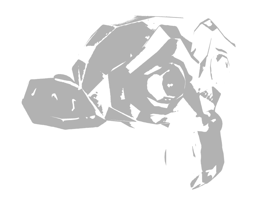
Here the grey represents the ground truth mesh, and the white is the very closely overlaid scanned mesh. As you can tell the surface triangles weave in and out of the other mesh, so they are quite closely aligned.

Now that both meshes are aligned, we need to compute the distance of each vertex of the scanned mesh to the entirety of the ground truth mesh. The algorithm is as follows to compute the distance of a point to a mesh:

1. For each vertex of the scanned mesh
   1. For each triangle of the ground truth mesh
      1. Determine the distance to the closest point of that triangle
   2. Determine the minimum distance to the ground truth mesh out of all the triangles
2. Determine the number of distances farther than 2% of the longest axis
3. Determine the number of distances farther than 5% of the longest axis
4. If the number of distances farther than 2% of the longest axis is more than 10% (100% – 90%) of the number of points, accuracy requirement has failed
5. If any distances are farther than 5% of the longest axis, accuracy requirement has failed.
6. Otherwise, verification has passed successfully, and accuracy requirements are met for the scan. Note that occlusion points are not considered since they can be accounted for by performing single-object multiple-scans using ICP.

This looks good, but the double for loop incurs a significant performance cost. We are ignoring this cost since the speed of verification is not important to any of our requirements (this cost can be alleviated by the use of a kd-tree or similar to partition the triangles into a hierarchy).

Finally, we are left with the question of how we can determine the distance of a point to the closest point on a triangle. The procedure to do this is to project the point onto the plane of the triangle, then determine which region of the triangle the point is in on the plane, and finally based on that region perform the correct computation. The regions are illustrated below for the 2D case:

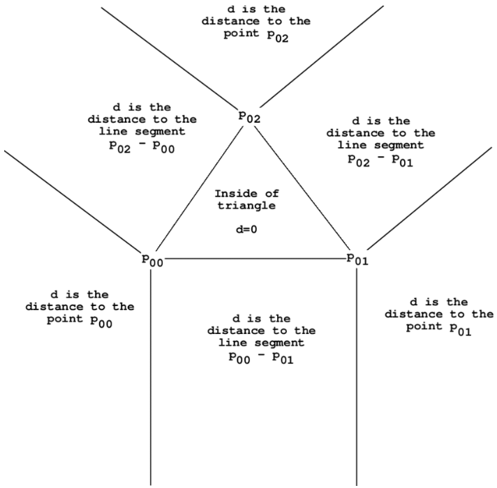
The computation is as follows for each of these cases:

1. Inside the triangle, the point distance is the distance from the point to the plane
2. To the line segment, the distance is the hypotenuse of the distance to the plane and the distance from the point on the plane to the line segment. This distance is computed by subtracting the portion of the vector from the projected point to a vertex that is parallel to the segment.
3. To a point of the triangle, the distance is the hypotenuse of the distance to the plane and the distance from the point on the plane to the point of the triangle.

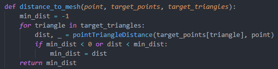
There were a couple implementation hurdles, such as figuring out how to extract triangle data from the mesh object. Specifically, the triangles property is an array of 3-tuples where each element corresponds to an index to a vertex in the vertices array. In this way triangles can be reconstructed by utilizing both of these arrays. Below is a sample of code to perform the distance computation from a point to a mesh, the point to triangle computation is quite complicated and is not posted here:

With all of this now implemented, we can perform verification of our scans to check that they meet the accuracy requirements. However, this verification process takes a significant amount of time, so I may in the next week optimize it to use a tree data structure.

My part of the project is on schedule for now, and at this moment we are preparing some examples for our in-lab demo on Monday. This next week I hope to optimize the verification process, test on a larger datasets of multiple objects, and overall try to optimize and streamline the scanning and verification processes. I do not see significant risks at the moment as our scans so far are meeting the accuracy requirements. I will also plan to acquire significant data regarding how accurate our scans are, and compile that data into a form that we can analyze to determine what weaknesses our current system has.

This week, our team focuses mainly on improving and making necessary fixes to our project. We also worked on preparing for the demo, by coming up with different test cases to show that we are achieving the requirements we have. We also discussed how to mimic issues that could potentially happen in the real world since we are using a simulation instead and will be working on that. We are also writing the testing code to compare the mesh we output and the ground truth mesh in order to output metrics that we can check against our accuracy requirements. 

 

Currently, there are no significant risks. 

 

There were no changes made to the existing design of our system. 

 

Below is the updated Gantt chart. 

https://docs.google.com/spreadsheets/d/1GGzn30sgRvBdlpad1TIZRK-Fq__RTBgIKN7kDVB3IlI/edit#gid=1867312600