Ryan’s status report for Saturday, Apr. 25

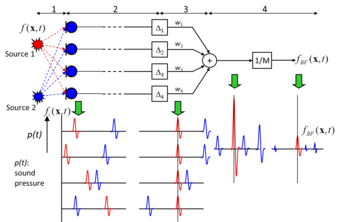
In Matlab, Sarah and I wrote the algorithm for beamforming using the sum & delay method. A simplified block diagram is shown below:

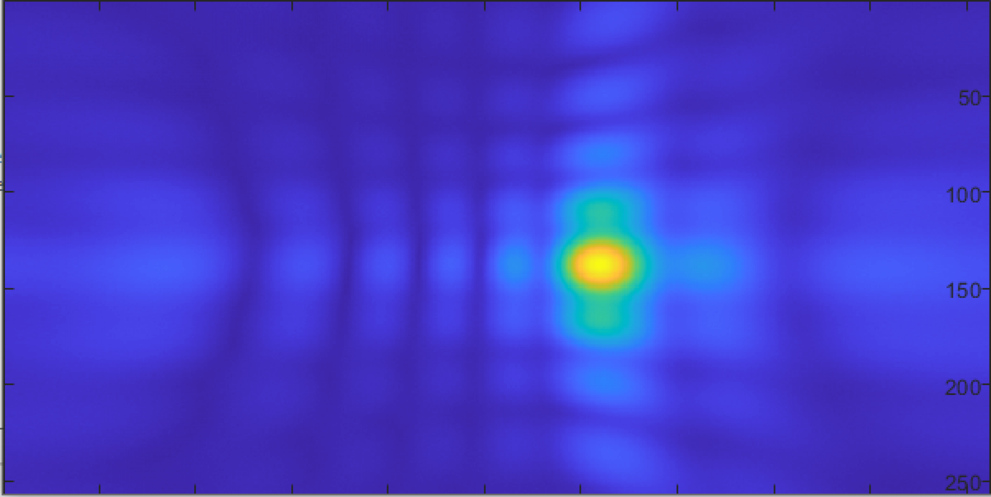
When we have an array of microphones, because of the distance differences between each microphone and the source, we can “steer” the array and focus on a very specific spot. By sweeping the spot over the area of interest, we can identify from where the sound is coming from. 

The “delay” in sum and delay beamforming is attributed to delaying the microphone output for each microphone depending on its distance from the sound source. The signals with appropriate delays applied are then summed up. If the sound source matches the focused beam, the signals constructively interfere and the resulting signal will have a large amplitude. On the other hand, if the sound source is not where the beam is focused, the signals will be out of phase with each other, and a relatively low amplitude signal will be created. Using this fact, the location of a sound source can be mapped without physically moving or rotating the microphone array. This technology is also used in 5G communications where the cell tower uses beamforming to focus the signal onto the direction of your phone for higher SNR and throughput. 

Ryan’s status report for Saturday, Apr. 18

This week, I was planning to analyze recordings from a 4×4 microphone array for sensitivity variances over frequency. Unfortunately we were having some trouble converting the captured PDM signals to a PCM wav file, and I did not have much time to look into this.

Next week, I’ll investigate this issue, and once we have the PCM wav recordings, I should be able to generate a EQ profile for each microphone for accurate level matching between them.

Ryan’s Status Report for Saturday, Apr. 11

I’m waiting for the 96 microphones to be assembled. Once all of them are functional, I’m going to calibrate them by having John capture their output with a sound source of three tones at 2563Hz, 8667Hz, and 12597Hz.  These three frequencies we were observed from the recording of the air leak, so we will focus on these.

The sound will be played through a bluetooth speaker approximately 8-10ft away from the microphone array to minimize the variations in distances between the microphone and the sound source. If the speaker were much closer, the angle between the microphone array and the speaker will have a larger variance, as well as the distance between the mic and the speaker, since the microphone array is flat, not curved.

In the microphone’s datasheet, it lists the maximum sensitivity variation to be +/- 1dB, so they should be pretty close to each other.

The most basic calibration will involve taking the average of the three tones’s output level and simply adding or subtracting an offset to compensate for the sensitivity of the microphone.

If we find significant differences in sensitivity from one microphone to the next depending on the frequency, we will have to generate an equalization factor that is dependent on frequency, such as in a graphic EQ.

Next week:

Get the microphone array assembled and perform the calibration procedure.


Ryan’s Status Report for Saturday, Apr. 4

This week I continued my work on synthesizing sounds of air leaks. I used a recording of a real air leak, performed an FFT on it, identified the peak frequencies in the audio, and created various variants of it.

As mentioned in last week’s update, the three peeks are at the following frequencies and amplitudes:

2563Hz: -24dB

8667Hz: -18dB

13597Hz: -17dB


I created waveforms of pure sine tone at 2563, 8667, and 13597Hz in three separate WAV files.

If all goes well, the phased array should be able to detect and physically locate the first two tones. The third tone’s wavelength is shorter than the distance between each microphones in the array, so it would be aliased. This is outside our frequency specification range, so the device should filter it out to prevent aliasing artifacts from appearing.


Next, I generated a Gaussian-distributed noise source centered at  approximately 2563, 8667, and 13597Hz in three separate WAV files.

They have the following frequency distributions:

They sound like this, in the order of increasing frequency:

The noise floor isn’t audibly low, and this is intentionally done to best match real world environments. If all goes well, the system should be able to detect and locate the first two tones even with the high noise floor.

Further work:

Reflow the 96 microphones and auxiliary components into the PCB and hook them up to the FPGA.

Test the system with the synthesized frequencies.

Ryan’s Status Report for Saturday, Mar. 28

This week I’ve worked on synthesizing a recording of an air leak for use in our performance testing and validation.

First, I downloaded an air leak sound effect and imported it in Audacity:

I then amplified it and kept only the middle portion where the leak noise was consistent:

I did an FFT to get an idea of the main frequency content:

We have peaks in the following locations:

2563Hz: -24dB

8667Hz: -18dB

13597Hz: -17dB

I then created an EQ profile to apply to a white noise source:

After applying the EQ to white noise, we get an FFT:

This looks very close to our original leak. We can use this synthesized sound to test the system after we verify it with a single tone sine wave. The synthesized source can act as an intermediary between the single tone and a real recording of a leak because this is more complex than a single tone, but less complex than the sound of a real leak.

Further work:

Deeper analysis into what sounds the system detects well and which sounds the system does not perform well with, and why.

Compare and contrast real world air leak recordings and synthesized versions.

Ryan’s Status Report for Saturday, Mar. 21

After talking to Patrick from TDK Invense, we were able go get 110 of the ICS-41351 from them. We’re very thankful for this because this would have been the most expensive part of the project, as shown below in the bill of materials from the design report:

If we were to order the microphones from Mouser, it would have costed $124.30. Now, we’re able to allocate that for monetary slack, as we may encounter situations during the build process that we may need to order new parts.


The candidates for the microphones were ICS-41351, INMP521, and INMP522. The latter two had slight better frequency response at the frequency of interest (5kHz and above), but we ultimately decided on the ICS-41351 because it had a footprint that was much nicer to work with.

It has relatively large pads on the bottom:

Because it has the microphone port on the top, the bottom solder pads are not constrained.

The INMP521 and the INMP522 however, have the microphone ports on the bottom, so it becomes  much more challenging to solder properly, because the solder ring around the port has to be completely soldered for best acoustic performance, and it’s not easy to verify proper soldering when we do not have access to professional reflow tools.

The main task moving forward is to get the PCBs that John designed made and reflow them. I think it’ll be a fun challenge.

Ryan’s Status Report for Saturday, Mar. 14

This week, we’ve worked on creating the FIR filter for converting the 1-bit 1-3MHz Pulse Density Modulation output of the microphone to a standard double precision array in MATLAB. Essentially, the FIR filter is a lowpass filter that only allows signals below 20kHz (human hearing range) to pass through.

We used MATLAB’s Filter Designer tool to generate a lowpass FIR filter with 1.000MHz sampling frequency, 20kHz passband, 25kHz stopband. The resulting FIR filter had 506 taps. I could have lowered the stop band at the expense of higher filter order, but I didn’t want to slow the system down too much during the actual filtering process. We will see if a sharper filter is needed. The FIR filter has the following frequency and phase response:

In order to apply the filter, we perform a convolution of the signal with the coefficients of the filter.

Original PDM signal, zoomed in:

Filtered result:

Filtered result, zoomed in:

Great, we are getting our 850Hz tone that we applied to the mic back!

Further considerations:

  • The process of convolving the PDM signal with the FIR filter seems to take a few seconds in MATLAB. We will need to optimize this for a realistic processing time for all 96 microphones.
  • I was not able to get the resulting signal’s audio to play in MATLAB. I do hear some pops and crackles though, so there must be a way to play a double array.
  • In talks with Patrick from TDK Invensense for microphones. We may be able to source the microphones from them instead of Mouser or Digikey, saving us a lot of money.


Team Status Update for Saturday, Feb. 29

We’re continuing our investigation with implementing 1Gbps Ethernet with our FPGA. The Spartan 6 board does come with two Gigabit Ethernet ports, but since it’s not a development board (actually an LED array controller), the Broadcom transceiver does not have a public datasheet for it, so it’s hard to control, even though it’s using the industry-standard RGMII protocol.

Instead, we’re looking into an expansion board with the Realtek RTL8211E from Numato. It has very good documentation that should make implementation much easier:


The output of the PDM microphone is a 1-bit digital signal. Even if the output is 1-bit high quality audio can be transmitted due to the fact that oversampling is occurring. For example, refer to this diagram below (Wikipedia):

If we average (low pass filter) the PDM signal in blue, we’re able to recover the original analog signal. Implementing a low pass filter with discrete analog components is one way to recover the audio, but since we’re dealing with 96 microphones, we want the processing to be digital for greater flexibility and we don’t need ADCs as well.

If performance turns out to be an issue, we will look into more efficient low pass filter algorithms such as using cascaded integrated-comb filters.

As a quick sanity check, we were able to probe the output of the PDM microphone and apply the scope’s low pass filter to get the signal back:

Ryan’s Status Update for Saturday, Feb. 29

This week we focused on our Design Review Presentation.  The format was similar to our Proposal Presentation, but this time, we focused on the specifics of the implementation and zeroing in on our metrics and requirements.

We narrowed down on our use case for the Sonic Imager; we’re going to use it to detect air leaks in pneumatic systems. Before, we packaged this as a general purpose audio to image conversion device, but we agreed that having a specific use case would help us focus on achieving metrics related to it, as opposed to being mediocre at everything.


John and I were able to test the basic operation of the PDM microphone. The Teensy 4 was providing a 1MHz clock to the PDM mic, and was receiving the digital output from it. We played an 820Hz tone from my phone, and when we probed the output, we were able to see a pulse density modulated signal. Using the scope’s built in low pass filter, we were able to recover the 820Hz tone: (PDM output in yellow, LPF signal in purple)

I’m currently working on a script to convert the PDM output into PCM audio. I first started writing the script in Python, but I’ve run into issue with signal visualization and plotting on my environment (Ubuntu WSL on Windows and TKInter).

I’ve decided to switch to MATLAB for its versatile graphing options, although it may take more time to write code. I plan to finish the script tomorrow.

Here’s 500 samples (about 0.5ms) of PDM output plotted:

The method of converting PDM to PCM is to create a low pass filter, and MATLAB has a nice library for that.

We are on schedule, and next week I’ll see if there are higher performance and time-efficient filters to speed up processing. CIC filters perhaps?

Team Status Update for Saturday, Feb. 22

Currently the primary risks are:

  • Not being able to get the gigabit ethernet working.  Managing this mainly by addressing it first,as it’s likely to be one of the most challenging parts of the project.  If we’re unable to get it working, it’s best to know soon so we can switch to another interface as soon as possible.  Current primary contingency plans are:
  1. Use a Zynq board.  The Zynq chip has a built-in gigabit MAC, and, many reference designs using it.  This moves the complexity from this to setting up the Zynq itself, though that will most likely use existing tools from the vendor.
  2. Use a USB interface.  Either a fast micro controller with a USB interface such as the Teensy 4.0, or one of several development boards specifically designed for simple, high-speed USB interfaces, such as the CYUSB3KIT.
  3. Use an off-the-shelf board that already has an working example written for it, such as the Mimas A7 from Numato.
  • Some aspect of the microphones renders then unsuitable for this project.  We are managing this risk, again, by tackling it early.  We have already ordered some sample microphones from Digikey and rigged up a testing board in order to run some basic tests and get some hands-on experience with PDM, since none of us have ever used it.

The overall design is unchanged from the previous update.