
This week, I finished up the tutorial of the image-captioning model using the Flickr8k dataset. I decided not to train it so as to save my GPU quota for training our actual graph-description and graph identification models.
I also looked more in depth into how image labels should be formatted. If we use a tokenizer (such as the one from keras.preprocessing.text), we can simply store all of the descriptions in the following format:
1000268201_693b08cb0e.jpg#0 A child in a pink dress is climbing up a set of stairs in an entry way .
1000268201_693b08cb0e.jpg#1 A girl going into a wooden building .
1000268201_693b08cb0e.jpg#2 A little girl climbing into a wooden playhouse .
1000268201_693b08cb0e.jpg#3 A little girl climbing the stairs to her playhouse .
Another thought I had about reference descriptions was whether it would be better to have all reference descriptions follow the same format, or have varied sentence structure. Since the standard image captioning problem typically requires captioning a more diverse set of images (as compared to our graph description problem), there is not much guidance on tasks similar to this. Inferring from image captioning, I think that a simpler/less complex dataset would benefit from a consistent format, and this also addresses the need for precise, unambiguous descriptions (as opposed to descriptions that would be more “creative”). This is why I think we should do an ablation study where we have maybe 3 captions per each image that will differ, and then either 1) follow the same format for all images, or 2) follow a different format for each image. Here is an example of the difference on one of the images:
Ablation Case 1:
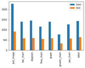
This is a bar graph. The x-axis displays the type of graph, and the y-axis displays the count for training and test data. The highest count is just_image, and the lowest count is growth_chart.
Ablation Case 2:
This bar graph illustrates the counts of training and test graphs over a variety of different graphs, including just_image, bar_chart, and diagram.
As you can see, the second case has more variation. We might want to have a balanced approach since we have multiple reference descriptions per image, so some of them can always have the same format, and others can have variation.
Unfortunately, it looks like the previous Kaggle dataset we found includes graph and axis titles in a non-English language, so we will have to find some new data for that.
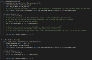
Additionally, I looked into the algorithm which will detect bounding boxes around the specific types of graphs we are interested in from a slide. I wrote some code which should be able to do this – the main architecture includes a backbone, a neck, and a head. The backbone consists of the primary CNN, which will be something like ResNet-50, and will give us feature maps. Then we can build a FPN (feature pyramid network) for the neck, which will essentially sample layers from the backbone, as well as perform upsampling. Finally, we will have 2 heads – a classification head and a regression head.
The first head will perform classification (is this a graph or not a graph?) and the second head will perform regression to identify the 4 coordinates of the bounding box. There is also code for anchor boxes and non-max suppression (which eliminates anchor boxes with a high enough IoU, so that we are not identifying 2 bounding boxes for the same object).
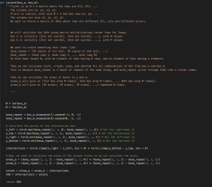
Here is some of the code I worked on.
My progress is almost caught up as I got through the tutorial, but I do still need to find new graph data, generate reference descriptions with my teammates, and train the CNN-LSTM. However, I also started working on the graph detection algorithm above ahead of schedule. My plan for the next week is to work on data collection as much as possible (ideally every day with my teammates) so that I can begin training the CNN-LSTM as soon as possible.