In performing engineering analysis and design, it is essential to communicate ideas clearly. One of the keys to communicating clearly is to present professional engineering graphics. "A picture is worth 1,000 words and equations …"
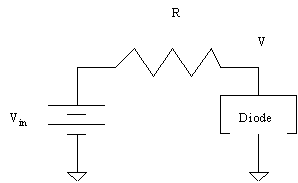
In this example, we will explore a circuit with a resistor and a diode, in series to a battery.

The equation for the current through the diode can be written as:
![]()
Writing KCL, and defining the current i flowing from left to right through the resistor, leads to:
![]()
Our goal is to find the operating point. We can use MATLAB to find the operating point. We first plot the equation for the current through the diode, and superimpose the equation obtained by using KCL. We define all parameters in MATLAB. While it is very easy to simply enter each of the commands needed for this exercise from the MATLAB command line, this demonstration will show how to create a MATLAB m-file to be used in a scripting nature.
Remember that it is important to comment MATLAB code, and thus all lines that begin with a % are comments.
The MATLAB script is located in: /afs/ece/class/ee205/public_html/resource/demonstration/plot_demo.m
The corresponding graphics are found in: /afs/ece/class/ee205/public_html/resource/demonstration/{plot_demo_1.ps, plot_demo_2.ps, plot_demo_3.ps}
(Ghostscript or other post script viewers may be used to view these plots.)
The diary file, a record of all commands and scripts executed is located in: /afs/ece/class/ee205/resource/demonstration/plot_demo.txt
The MATLAB script is included below for convenience:
% plot_demo.m
%	This file contains a brief demonstration of MATLAB plotting

% %%%%%%%%%%%%%%%%%%%%%%%%%%%%%%%%%%%%%%%%%%%%%%%%%%%%%%%%%%%%%%%%%%%%%%%%
%     Title:	ps1.m
%   Created:	Tuesday, January 20, 1998
%   Project:	18-205, Mathematical Software in Engineering, Spring 1998
%   Purpose:	Demonstrate a variety of MATLAB plotting commands
% 		and the use of an m-file as a script.
% %%%%%%%%%%%%%%%%%%%%%%%%%%%%%%%%%%%%%%%%%%%%%%%%%%%%%%%%%%%%%%%%%%%%%%%%

% Just as commands can be entered on the command line, commands
% can be entered in a script file.  When performing analysis it
% is often easier to enter the commands in a script file, and
% rerun the file (rather than retype a variety of commands).

% This file analyzes a circuit with a resistor and a diode.
% The diode is characterized by the equation:
%	i = Io{Exp[beta*V] - 1}

% The KCL equation for the circuit is given by:
%	i = (Vin - V)/R

% Now, enter all required parameters:
Io = 100e-6	% Amps (100 microamps -- entered in scientific notation)
Vin = 5		% Volts
beta = 2	% diode characteristic
R = 1e3		% Ohms (choose a 1k-Ohm resistor for this analysis)
		% what happens when you change 1k to 10k?

% Choose a range of values of V to analyze the circuit over
V = -5:0.001:10;
% The result of the above command creates a vector of values to
% plot.  The first number in the sequence (-5) describes the value
% the vector should begin at.  The second number in the sequence
% (0.001) indicates the step size.  The final number indicates
% the end of the range (10).  Thus, the above line creates a vector
% starting at -5V in increments of 0.001V to 10V.  The step size
% must be controlled so as to obtain the correct output (too many
% or too few points are not good)

% Compute values for i from the diode equation.
i1 = Io.*(exp(beta.*V) - 1);
% Note the use of the .* operator.  This indicates to multiply
% each element in the vector V, and not perform vector multiplication.

% Determine the values for i from the KCL equation.
i2 = (Vin - V)./R;
% Note the ./ operator in the above function.  Also note in the above
% three equations, a ";" was placed at the end of the line.  This
% supresses the output of the function or operation.

% Now, plot the data.
plot(V,i1,V,i2);

% Whenever a plot is created, it is useful to label the plot as:
xlabel('Voltage (V)');
ylabel('Current (A)');
title('Current as a function of Voltage for Series Resistor-Diode Circuit');
legend('i1 (diode equation)','i2 (KCL equation)');

% use the axis command to zoom in on the data
axis([-2,2,-100e-3,100e-3]);

% you might have to try more than once
print plot_demo_1.ps
disp('press any key to continue');
pause
axis([1,2.5,-10e-3,10e-3]);

disp('now use the zoom command, and the ginput command to obtain');
disp('the intersection values of the two lines');

% end of file
The m-file above was run, and the output was recorded in the diary file. To start a diary file, type the command diary on.
>> plot_demo
Io =
   1.0000e-04
Vin =
     5
beta =
     2
R =
        1000
press any key to continue
now use the zoom command, and the ginput command to obtain
the intersection values of the two lines
>> print plot_demo_2.ps
>> zoom on
>> zoom off
>> ginput
ans =
    1.7550    0.0032
>> print plot_demo_3.ps
>> diary off
The key points to take away from this demonstration:
This page was last updated on Tuesday, January 20, 1998.
Send questions, comments, ideas, suggestions, or concerns to jsilvey@ece.cmu.edu.
18-205 Web Resources 1998
Carnegie Mellon University
Department of Electrical and Computer Engineering