Jonathan’s Status Update for Saturday April 25
This week I mainly finished the hardware and continued refining the real-time imaging.
The hardware was half completed at the beginning of this week, with 48 microphones assembled on their boards and tested. At the beginning of this week I assembled the remaining 48.
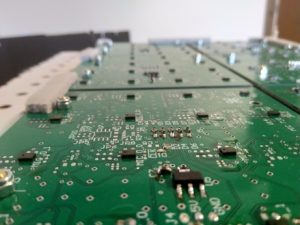
Since the package for these microphones, LGA_CAV, are very small, with a sub-mm pitch, and no exposed pins, soldering was difficult and often required rework. Several iterations of the process to solder them were used, beginning with a reflow oven, eventually moving to hot air and solder past, then manual tinning followed by hot air reflow. The final process was slightly more time consuming than the first two, but significantly more reliable. In all, around 20% of the microphones had to be reworked. In order to aid in troubleshooting, a few tools were used. The first was a simple utility I wrote based on the real-time array processor, which examined each microphone for a few common failures (stuck 0, stuck 1, “following” its partner, and conflicting with its partner).
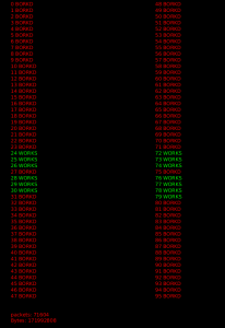
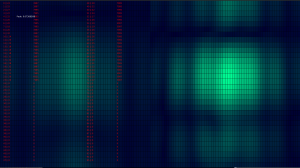
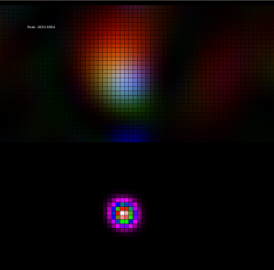
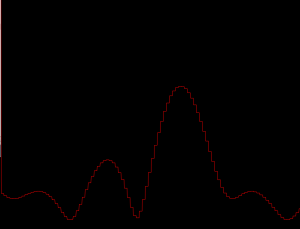
This image shows the output of this program (the “bork detector”) for a partially working board. Only microphones 24-31 and 72-79 are connected (a single, 16-microphone board), but 27,75, and 31 are broken. This enabled quickly determining where to look for further debugging.
The data interface of PDM microphones is designed for stereo use, so each pair takes a single clock line, and has a single digital output for both. Based on the state of another pin, each “partner” outputs data either on the rising or falling edge of the clock, and goes hi-z in the other clock state. This allows the FPGA to use just half as many pins as there are microphones (in this case, 48 pins to read 96 microphones). Often the errors in soldering could be figured out based on this.
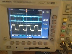
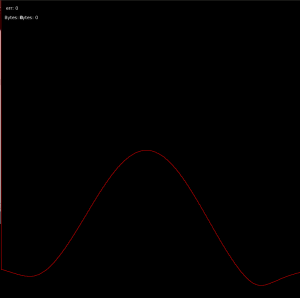
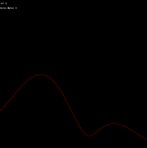
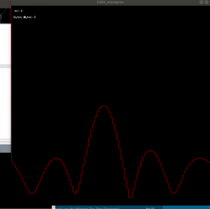
Using an oscilloscope, a few common errors could quickly be identified, and tracked to a specific microphone, by probing the clock line and data line of a pair (blue is data, yellow clock):
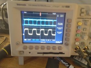
Both microphones are working
The falling-edge microphone is working, but the data line of the rising-edge microphone (micn_1) is disconnected
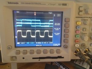
The falling-edge microphone is working, but the rising-edge microphone’s select line is disconnected.
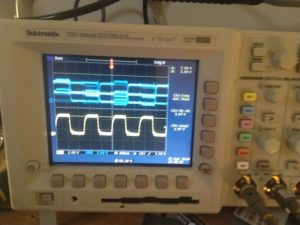
The falling-edge microphone is working, but the rising-edge microphone’s select line is connected to the wrong direction (low, where it should be high).
The other major thing that I worked on this week was refinements to the real-time processing software. The two main breakthroughs here that allowed for working high-resolution, real time imaging was using a process which I’ll refer to as product of images (there may be another name for this in the literature or industry, but I couldn’t find it), and frequency-domain processing.
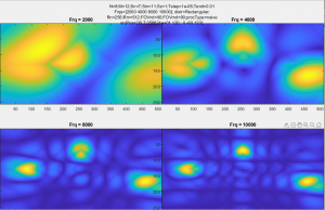
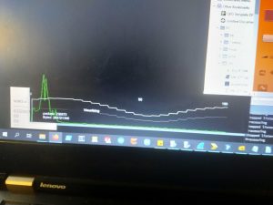
Before using product of images, the images generated by each frequency were separate, as in this image where two frequencies (4000 and 6000Hz) are shown in two images side by side:
Neither image is particularly good on its own (this particular image also used only half of the array, so the Y axis has particularly low gain). They can be improved significantly by multiplying two or more of these images together though. Much like how a Kalman filter multiplies distributions to get the the best properties of all the sensors available to it, this multiplies the images from several (typically three or four) frequencies, to get the small spot size of the higher frequencies, as well as the stability and lower sidelobes of lower frequencies. This also allows a high degree of selectivity, a noise source that does not have all characteristics of the source we’re looking for will be reduced dramatically.
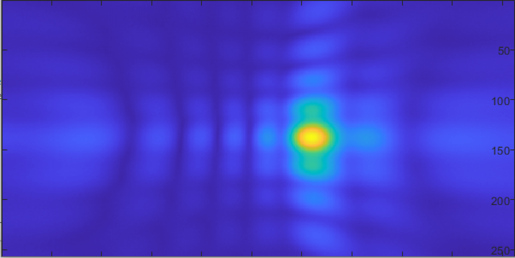
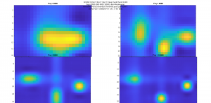
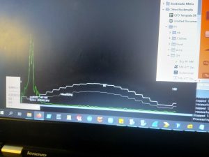
For a simple example, suppose we have a fan that has relatively flat (“white”) noise from 100Hz – 5KHz, and 10dB lower noise above 5KHz (these numbers based roughly on the fan in my room). If the source we’re looking at has strong components at 2,4,6,and 8 KHz, and the two have roughly equal peak signal power, then “normal” time domain processing that adds power across the entire band would have the fan be vastly more powerful than the source we’re looking for, as the overall signal power would be greater because of the very wide bandwidth (4.9KHz bandwidth as opposed to just a few tens of Hz, depending on the exact microphone bitrate). Doing product of images though would have the two equal at 2 and 4KHz, but would add the 10dB difference at both 6 and 8KHz, in theory giving a 20dB SNR over the fan. This, for example, is an image created from about 8 feet away, where the source was so quiet my phone microphone couldn’t pick it up more than 2-3 inches away:
In practice this worked exceptionally well, largely cancelling external noise, and even some reflections, for very quiet sources. Most of the real-time imaging used this technique, some pictures and videos also took the component images and mapped each to a color based on its frequency (red for low, green for medium, blue for high), and just made an image based on these. In this case, artifacts at specific frequencies were much more visible, but it did give more information about the frequency content of sources, and allowed identifying sources that did not have all the selected frequencies. In the image above, the top part is an RGB image, the lower uses product of images.
Finally, frequency domain processing was used to allow very fast operation, to get multiple frames per second. Essentially each input channel is multiplied by a sine and cosine wave, and the sum of each of those waves over the entire input duration (typically 50mS) is stored as a single complex number. So for a microphone, if f(t) is the reading (1 or -1) at time t, and c is the frequency we’re analyzing divided by the sample rate, then this complex number is given by f(0)*cos(c*0) + f(1)*cos(c*1) … + f(n)*cos(c*n) + f(0)*sin(c*0)*j + f(1)*sin(c*1)*j + f(n)*sin(c*n)*j. Once all of these are computed, they’re approximately normalized (any values too small are kept small, larger values are kept relatively small, but allowed to grow logarithmically). To generate images, a phase table, which was precomputed when the program first started, is used to map a phase offset for each element, for each pixel. This phase delay is proportional to the frequency of interest, and what the time delay would have been if we were doing time domain delay-and-sum. Each microphone’s complex output value is multiplied by a value with this phase and magnitude 1, and then those numbers are summed, and the amplitude taken, to get a value for that pixel in the final image. While significantly more complicated than delay-and-sum, and much more limited as it can only look at a small number of specific frequencies, this can be done very quickly. The final real-time imaging program was able to achieve 2-3 frames per second, where post-processing in the time domain typically takes several seconds (or even minutes, depending on the exact processing method being used).
Team status update for Saturday April 25
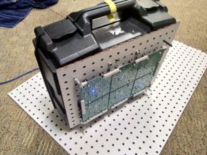
This week saw the completion of all major parts of the project. The hardware is finished:
And software is working:
John worked mainly on finishing the hardware, completing the remaining half of the array this week, Sarah and Ryan on the software, generating images from array data.
Going forward, we mainly plan to make minor updates to the software, primarily to make it easier to use and configure. We may also make minor changes to improve image quality.
Team status report for Saturday April 18
This week we made significant headway towards the finished project. The first three microphone boards are populated and tested, and most of the software for real-time visualization and beamforming has been written. At this point, we all have our heads down, finishing our portion of the project, so most of the progress this week has been detailed in individual reports. There were some hiccups as we’re expanding the number of operational microphones in the system, but that should be fixed next week.
This coming week, we’ll all continue working on our respective parts, planning to finish before the end of the week. John will mainly be working on finishing the hardware, and Ryan and Sarah, the software.
We are roughly on track with regards to our revised timeline, the hardware should be done within a few days, and all the elements of the software are in place and just need to be refined and debugged.
Jonathan’s status report for Saturday, Apr. 18
This week I mainly worked on improving the real-time visualizer, and building more of the hardware.
The real-time visualizer previously just did time-domain delay and sum, followed by a Fourier transform of the resulting data. This worked but is slow, particularly as more pixels are added to the output image. To improve the resolution and speed, I switched to taking the FFT of every channel immediately, then, only at the frequencies of interest, adding a phase delay to each one (which is computed ahead of time), then summing. This reduces the amount of information in the final image (to only the exact frequencies we’re interested in), but is extremely fast. Roughly, the work for delay-and-sum is 50K (readings/mic) * 96 (mics) per pixel, so ~50K*96*128 multiply-and-accumulate operations for a 128-pixel frame. With overhead, this is around a billion operations per frame, and at 20 frames per second, this is far too slow. The phase-delay processing needs only about 3 (bins/mic) * 8 (ops / complex multiply) * 96 (mics) * 128 (pixels), which is only about 300K operations, which any computer could easily run 20 times per second. This isn’t exact, it’s closer to a “big O” for the work number than an actual number of operations, and doesn’t account for cache or anything, but does give a basic idea of what kind of speed-up this type of processing offers.
I did also look into a few other things related to the real-time processing. One was that since we know our source has a few strong components at definite frequencies, is multiplying the angle-of-arrival information of all frequencies together gives a sharper and more stable peak in the direction of the source. This can also account, to some degree, for aliasing and other spatial problems – it’s almost impossible for all frequencies to have sidelobes in exactly the same spots, and as long as a single frequency has a very low value in that direction, the product of all the frequencies will also have a very low value there. With some basic 1D testing with a 4-element array, this worked relatively well. The other thing I experimented with was using a 3D FFT to process all of the data with a single (albeit complex) operation. To play with this, I used the matlab simulator that I used earlier to design the array. The results were pretty comparable to the images that came out of the delay-and-sum beamforming, but ran nearly 200 times faster.
output from delay-and-sum.
output from 3D FFT
The two main disadvantages are that the 3D FFT has a fixed resolution output-the same as the physical array (8×12). To increase the resolution slightly, I wrote a bit of code to do complex interpolation between pixels. This “recovers” some of the information held in the phase of the output array, which normally would not be used in an image (or at least, not in a comprehensible form), and makes new pixels using this. This is relatively computationally expensive though, and only slightly improves the resolution. Because of the relative complexity of implementing this, and the relatively small boost in performance compared with phase-delay, this will probably not be used in the final visualizer.
Finally, the hardware has made significant progress since last week, three out of the six microphone boards have been assembled, and tested in a limited capacity. No images have been created yet, though I’ve taken some logs for Sarah and Ryan to start running processing on some actual data. I did do some heuristic processing to make sure the output from every microphone “looks” right. The actual soldering of these boards ended up being a very significant challenge. After a few attempts to get the oven to work well, I decided to do all of them by hand with the hot air station. Of the 48 microphones soldered so far, 3 were completely destroyed (2 by getting solder/flux in the port, and 1 by overheating), and about 12 did not solder correctly on the first try and had to be reworked. I plan to stop here for a day or two, and get everything else working, before soldering the last 3 boards.
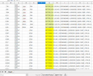
Finally, the FPGA firmware was modified slightly. Previously, timestamps for each microphone reading were included in the packets, to find “breaks” (dropped packets/readings) between readings in the packet handling, logfiles, or processing code. Since all of that is working reliably at this point, and that introduced significant (32Mbps) overhead, I’ve removed the individual timestamps and replaced it with packet indexing, each packet has a single number which identifies it. In this way missing packets can still be identified, but with very little overhead. The FPGA also now reads all 96 microphone channels, simultaneously, where previously it only read a single board. Since this required many pins, and the exact pinout may change for wiring reasons, I made a spreadsheet to keep track of what was connected where, and used this spreadsheet to automatically generate the .ucf file for all the pins based on their assignments within the sheet.
Team status report for Saturday April 11
This week started with the midpoint demo, which worked relatively well, showing mainly the real-time visualization shown in one of the previous updates. During the remainder of the week significant progress was made in several areas, particularly the network driver, which was previously impeding progress on the processing software.
Some progress on the hardware was also made (see John’s update), with the first board getting several microphones populated, tested, and hooked up to the FPGA. With this, we have finally moved from proof-of-concept tools, and started using the final hardware-firmware-software stack. Though these parts will of course be modified, at this point, there is no longer anything entirely new to be added.
Jonathan’s Status Report for Saturday, Apr. 11
This week I mainly worked on the network driver and microphone board hardware.
Last week, there was a problem that emerged with the network driver dropping up to 30% of the packets being transmitted from the FPGA, I spent most of this week working on resolving that. The library being used previously was the “hypermedia.net” java library, which works well for low-speed data, but does not buffer packets well, and this was causing most of the drops. By switching to linux and using the regular C network library, this problem was eliminated, though it required rewriting the packet processing and logging code in C.
The next problem was moving this data to a higher-level language like java, python, or matlab to handle the graphics processing. Initially, started looking into ways to give both programs access to the same memory, but this was complicated, not very portable, and difficult to get working. Instead, I ended up deciding on using linux pipes/fifos, as they use regular file I/O, which c and java of course support very well. One small problem that emerged with this had to do with the size of the fifo, which is only 64kB. The java program had some problems with latency relative to the C program, so the FIFO was getting filled, and it was dropping readings. To get around this, I modified the C program to queue up 50,000 readings at once, and put them into a single call to fprintf, and the java program reads in a similar way before processing any of the readings. In this way, the overall throughput is improved, by having just 20 large, unbroken transfers per second, rather than several thousand smaller ones. This does introduce some latency, though only 1/20th of a second which is easily tolerable, and takes more memory, but only a few megabytes.
Progress on the hardware has mainly been in figuring out the process for manufacturing all the microphone boards. There were initially some problems with the reflow oven blowing microphones off the board while the solder was still molten. The fan used to circulate air to cool the chamber after it has reached its peak temperature has no speed control, and is strong enough in some areas to blow around the relatively large and light microphones. So far, I have gotten the first few test microphones to work by reflowing them by hand with hot air, which worked but took a significant amount of work per microphone, so it may not be a viable solution for the whole array. I have started working on adding speed control and/or flow straighteners to the reflow oven fan as well, though I suspect I’ll be in for a long day or two of soldering.
With the working test board, I was able to use the real-time visualizer to do some basic direction finding for a couple of signals, which were extremely promising:
5KHz, high resolution, centered in front of the array (plot is amplitude vs direction)
5KHz, high resolution, off-center (about 45 degrees)
Low resolution, 10KHz centered in front of the array
10KHz, low resolution, about 15 degrees off center.
Next week I mainly plan to focus on the hardware, mainly populating all of the microphones and making the wiring to the FPGA.
Team Status Update for Saturday, Apr. 4
This week significant progress made in all areas of the project, including the hardware/FPGA component catching back up to the planned timeline.
To prepare for the midpoint demo on Monday, all group members have been working on getting some part of their portion of the project to the point where it can be demonstrated. John has a working pipeline to get microphone data through the FPGA and into logfiles, Sarah has code working to read logfiles and do some basic processing, and Ryan has developed math and code that works with Sarahs to recover the original audio.
While at this point the functionality only covers basic direction-finding, this bodes well for the overall functionality of the project once we have more elements and therefore higher gain, directionality, and the ability to sweep in two dimensions. The images below show basic direction-finding, with sources near 15 degrees from the element axis (due to the size of the emitter, placing it at 0 was impossible), and near 90 degrees to the elements. The white line plots amplitude over angle, and so should peak around the direction of the source, which it does:
~15 degrees:
~90 degrees:
This coming week should see significant progress in the hardware, as we now have all materials required, continued refinement of the software, as most of the major components are now in place.
Jonathan’s Status Report for Saturday, Apr. 4
This week I mainly worked on updating the FPGA firmware and computer network driver. Boards arrived yesterday, but I haven’t had time to begin populating them.
Last week, the final components of the network driver for the FPGA were completed, this week I was able to get microphone data from a pair of microphones back from it, do very basic processing, and read it into a logfile. This seemed to work relatively well:
source aligned at 90 degrees to the pair of elements (white line peaks near 90 degrees, as it should)
source aligned at 0 degrees to the pair of elements (white line has a minimum near 90 degrees, again as it should)
However, these early tests did not reveal a problem in the network driver. Initially, the only data transmitted was the PDM signal, which varies essentially randomly over time, so as long as some data is getting through, so it is very difficult to see any problems in the data without processing it first. Several days later when testing some of the processing algorithms (see team and Sarahs updates), it quickly became apparent that something in the pipeline was not working. After checking that the code for reading logfiles worked, I tried graphing an FFT of the audio signal from one microphone. It should have had a single, very strong peak at 5KHz, but instead, had peaks and noise all over the spectrum:
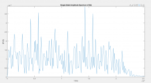
I eventually replaced some of the unused microphone data channels with timestamps, and tracked the problem down to the network driver dropping almost 40% of the packets. While Wireshark verified that the computer was able to receive them just fine, there was some problem in the java network libraries I had been using. I’ve started working on a driver written in C using the standard network libraries, but haven’t had time to complete it yet.
Part of the solution may be to decrease the frequency of packets by increasing their size. While the ethernet standard essentially arbitrarily limits the size of packets to be under 1500 bytes, most network hardware also supports “jumbo frames” of up to 9000 bytes. According to this : https://www.google.com/url?sa=t&rct=j&q=&esrc=s&source=web&cd=6&ved=2ahUKEwjrx8zAvM_oAhUvhXIEHcBHDmYQFjAFegQIBxAB&url=https%3A%2F%2Farxiv.org%2Fpdf%2F1706.00333&usg=AOvVaw1OaEu0ozlfTlaN1ZTfb-IW paper, increasing the packet size above about 2000 bytes should substantially lower the error rate. So far I’ve been able to get the packet size up to 2400 bytes using jumbo frames, but I have not finished the network driver in order to test it.
Next week I mainly plan to focus on hardware, and possibly finish the network driver. As a stop-gap, I’ve been able to capture data using wireshark and write a short program to translate those files to the logfile format we’ve been using.
Jonathan’s Status Report for Saturday, Mar. 28
This week I mainly worked on the microphone boards and FPGA drivers. The microphone boards were finished early this week, and ordered on Wednesday. They were fabricated and shipped yesterday, and expected to arrive by next Friday (4/3).
As mentioned previously, this design uses a small number of large boards with 16 microphones each, connected directly to the FPGA board with ribbon cables. This should significantly reduce the amount of work required to fabricate the boards and assemble the final device, though at the expense of some configurability, if we have to change some parameter of the array later.
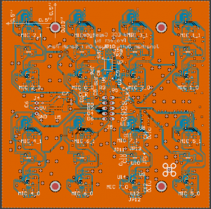
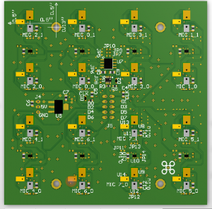
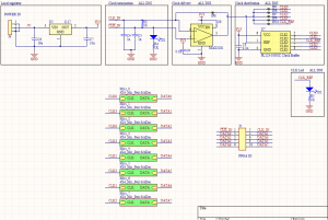
As the schematic shows, most of the parts on the board will not be populated, but were included as mitigations to possible issues. The microphone footprints were included in case we need to change microphones, and there are several different options for improving clock and data signal integrity (such as differential signaling and termination), if needed. Most parts, particularly the regulator, are relatively generic, and so can be acquired from multiple vendors, in case there is a problem with our digikey order (which was also placed this week).
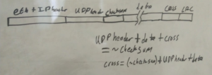
While working on the FPGA ethernet driver, one problem that came up was with the UDP checksum. Unlike the ethernet frame CRC, which is in the footer of the packet, the UDP checksum is held in the packet header:
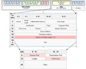
This means that the header depends on all of the data to be sent, which, means that the entire packet must be held in memory, then the checksum computed, then either the checksum modified in memory before transmission, or, during transmission the “source” of data has to be changed from memory to the register holding the checksum. I didn’t particularly like either of these solutions, and so, came up with another. I made the checksum an arbitrary constant, and added two bytes to the end of the UDP payload. Those two bytes, which I termed the “cross”, are computed based on all of the data, and the header, so that the checksum works out to that constant. The equation below isn’t exactly right, but gives the basic idea:
In this way, the packet can be sent out without knowing it’s entire contents ahead of time. In fact, if configured to do so, could actually take in new microphone data in the middle of the transmission of a packet, and include that in the packet. This greatly simplifies the rest of the ethernet interface controller, at the expense of a small amount of data overhead in every packet. Given the size of the packets though, this tradeoff is easily worth it.
This coming week, I mainly plan to work on getting the information flow, all the way from the FPGA PDM inputs to a logfile on a computer working. This was expected to be completed earlier, but the complexity of ethernet frames ended up being significantly greater than expected, and took several long days to get working. At this point all the components of the flow are working to some degree, but do not work together yet.