This week I mainly worked on improving the real-time visualizer, and building more of the hardware.
The real-time visualizer previously just did time-domain delay and sum, followed by a Fourier transform of the resulting data. This worked but is slow, particularly as more pixels are added to the output image. To improve the resolution and speed, I switched to taking the FFT of every channel immediately, then, only at the frequencies of interest, adding a phase delay to each one (which is computed ahead of time), then summing. This reduces the amount of information in the final image (to only the exact frequencies we’re interested in), but is extremely fast. Roughly, the work for delay-and-sum is 50K (readings/mic) * 96 (mics) per pixel, so ~50K*96*128 multiply-and-accumulate operations for a 128-pixel frame. With overhead, this is around a billion operations per frame, and at 20 frames per second, this is far too slow. The phase-delay processing needs only about 3 (bins/mic) * 8 (ops / complex multiply) * 96 (mics) * 128 (pixels), which is only about 300K operations, which any computer could easily run 20 times per second. This isn’t exact, it’s closer to a “big O” for the work number than an actual number of operations, and doesn’t account for cache or anything, but does give a basic idea of what kind of speed-up this type of processing offers.
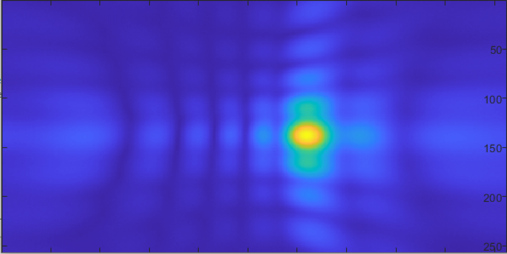
I did also look into a few other things related to the real-time processing. One was that since we know our source has a few strong components at definite frequencies, is multiplying the angle-of-arrival information of all frequencies together gives a sharper and more stable peak in the direction of the source. This can also account, to some degree, for aliasing and other spatial problems – it’s almost impossible for all frequencies to have sidelobes in exactly the same spots, and as long as a single frequency has a very low value in that direction, the product of all the frequencies will also have a very low value there. With some basic 1D testing with a 4-element array, this worked relatively well. The other thing I experimented with was using a 3D FFT to process all of the data with a single (albeit complex) operation. To play with this, I used the matlab simulator that I used earlier to design the array. The results were pretty comparable to the images that came out of the delay-and-sum beamforming, but ran nearly 200 times faster.
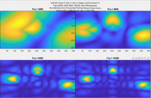
output from delay-and-sum.
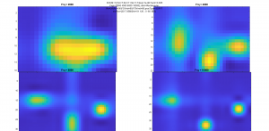
output from 3D FFT
The two main disadvantages are that the 3D FFT has a fixed resolution output-the same as the physical array (8×12). To increase the resolution slightly, I wrote a bit of code to do complex interpolation between pixels. This “recovers” some of the information held in the phase of the output array, which normally would not be used in an image (or at least, not in a comprehensible form), and makes new pixels using this. This is relatively computationally expensive though, and only slightly improves the resolution. Because of the relative complexity of implementing this, and the relatively small boost in performance compared with phase-delay, this will probably not be used in the final visualizer.
Finally, the hardware has made significant progress since last week, three out of the six microphone boards have been assembled, and tested in a limited capacity. No images have been created yet, though I’ve taken some logs for Sarah and Ryan to start running processing on some actual data. I did do some heuristic processing to make sure the output from every microphone “looks” right. The actual soldering of these boards ended up being a very significant challenge. After a few attempts to get the oven to work well, I decided to do all of them by hand with the hot air station. Of the 48 microphones soldered so far, 3 were completely destroyed (2 by getting solder/flux in the port, and 1 by overheating), and about 12 did not solder correctly on the first try and had to be reworked. I plan to stop here for a day or two, and get everything else working, before soldering the last 3 boards.
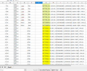
Finally, the FPGA firmware was modified slightly. Previously, timestamps for each microphone reading were included in the packets, to find “breaks” (dropped packets/readings) between readings in the packet handling, logfiles, or processing code. Since all of that is working reliably at this point, and that introduced significant (32Mbps) overhead, I’ve removed the individual timestamps and replaced it with packet indexing, each packet has a single number which identifies it. In this way missing packets can still be identified, but with very little overhead. The FPGA also now reads all 96 microphone channels, simultaneously, where previously it only read a single board. Since this required many pins, and the exact pinout may change for wiring reasons, I made a spreadsheet to keep track of what was connected where, and used this spreadsheet to automatically generate the .ucf file for all the pins based on their assignments within the sheet.