
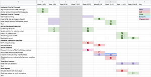
Team Status Update 4/26
This week was spent on collecting more data and visualizing it. We also worked on the final presentation.
Shiva continued to collect data from the hardware. Adding the warm up period before collecting the data improved it, and reduced the standard deviation.
Udit worked to improve the simulator, so we can have better reporting and visualization.
Rhea worked to tune the Kalman filter.
Next week we will be testing and collecting data from our simulator using real NBA data.
Rhea’s Status Update 4/26/2020
This week I worked on tuning the Kalman filter and the final presentation.
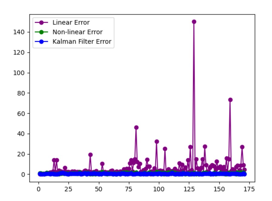
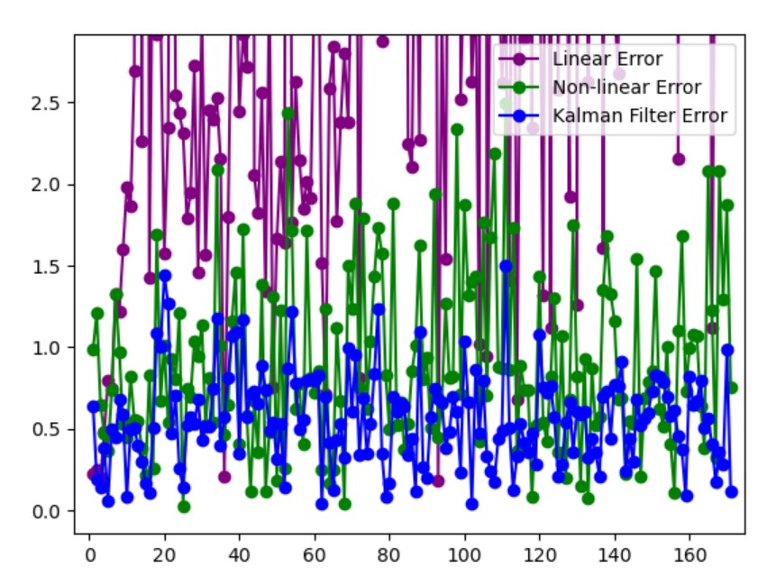
The filter performed better than the liner and non-linear localization. The RMSE for one of the runs was 15.223 m for linear, 1.065 m for non-linear, and 0.631 m for the filter.
Next week I will be working on updating the Kalman filter to work with the data sets that Udit will include in the simulation. I will probably attempt to have the predict step use the velocity of the tag, instead of using the current position.
Shiva’s Status Update for 04/26
This week, I worked on the final presentation and collected more data to help Udit and Rhea refine the multilateration algorithm:
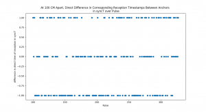
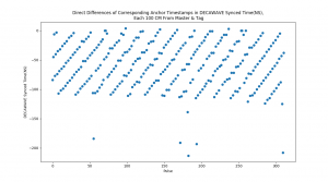
At Tamal’s recommendation, I let the anchors ‘warm up’ by running them continuously for at least 30 minutes prior to testing. This contributed to a significant reduction in timestamp reception variance in real-world testing, sampled below:
Test 10 — Stats of Direct Difference in Synchronized Reception Timestamps between Anchors that are equidistant from Tag, in Nanoseconds:
Mean = -0.11842105263157894,
Median = 0.0
St. Dev = 0.8105733069084967
—-
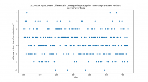
Test 11 – Stats of Direct Difference in Reception Timestamps between Anchors that are equidistant from Tag, in Nanoseconds:
Mean = 0.3470031545741325,
Median = 0.0,
St. Dev = 1.4427340556024508
We are on schedule for our presentation this week and demo + report next week. Next week, I will work on the report and, if needed, scale up the experiment for more anchors.
Team Status Report 4/19
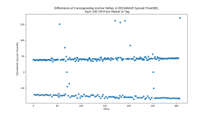
Shiva has been working on collecting experimental demo values for the hardware so that we can model them in the simulator. We actually got REALLY promising results with very low standard deviation and a very consistent pattern (after removing outliers).
This graph had a standard deviation of <1ns which again is really promising because it means if you assume a synchronized clock, the error from other hardware components is quite low! Plus, the very consistent shape of the graph (same shape in multiple trials) looked like the result of oscillator clock drift to us.
So we implemented a simple algorithm to sync slave anchors with a master clock to see if it would improve our results. Shiva managed to implement it, but we are still trying to process and interpret the results.
As soon as those results are ready, we should be able to incorporate them into the simulator that Rhea and Udit have been working on. Details of that are available on Udit’s status page.
We are hoping that we can get that integration done by the demo. We have collected so many data points and graphs that will at least make our Final Paper quite interesting.
Udit’s Status Report 4/19
So I had a pretty productive and interesting 2 weeks (missed last week’s update so will combine with this)
- By the end of last week, we came together and formalized our mathematical models. We are going to go with 3 approaches: System of Linear Eqs, System of Non-Lins, and an Extended Kalman Filter Smoothened model. I worked on implementing the former 2 options.
- Then I implemented that math with a visualizer for each type where the TDoAs from the simulated tag will get passed to the algorithms and they will spit out a value that gets visualized back on the map
- Rhea was able to add in the algorithm for Kalman filter as well
- Here is an image of what the live visualization. The black circle is the tag (real location), purple square is linear-algorithm calculated location, green square is hyperbolic-algorithm calculated location, and blue square is the kalman filter algorithm calculated location.
- Then for this week I worked on adding in error-reporting so that we can calculate the Root Mean Squared Error for each algorithm
- Also have exported all values to CSVs so that we can store logs for each file and play back the data. I will be adding in a separate program that reads this CSV and visualizes the real path taken and the path modeled (for the paper).
- Here is sample of results for a basic movement of the tag around the lines of hte basketball court.
- Our RMSE (in meters) for that sample run was the following:
- Lin RMSE: 3.8608529220466794
nonLin RMSE: 0.14847987088052897
filter RMSE: 0.11742101999581132 - This is really promising because it lines up with our general expectations that Linear<Non-linear<filtered
- Right now this test is with 4 anchors which only leaves 2 equations for the linear. Hopefully Linear numbers become a lot more usable with 6 anchors
- Lin RMSE: 3.8608529220466794
- Our RMSE (in meters) for that sample run was the following:
- I am awaiting finalized hardware error numbers from Shiva to add in artificial error
- I will also be looking for a dataset of player movements for real NBA games so we can get realistic movement of players/tags.
- I will try to run a BUNCH of variations of tests with multiple player paths (real-NBA and simulated), multiple anchor configurations, and multiple error simulations.
Rhea’s Status Update 4/19/2020
This week I got the extended Kalman filter working. We decided to use the filterpy library for the filter to save time in writing the filter, and focus on getting it to work. When I was starting, I ran into some issues with making sure I had the right dimensions for all the matrices. At first I was trying to do linear Kalman filter, but did it incorrectly, and realized that I used a measurement model wasn’t a constant. Since the measurement was nonlinear, I decided to work on the extended Kalman filter instead. The first time I tried to test the Kalman filter the positions it was estimating were very wrong, and realized that the equations I was using for the measurement model were incorrect. Once I fixed the equations, I ran into a few other issues where I was using the wrong variable names for certain things. After I fixed those last few bugs, we had a working extended Kalman filter.
Our current simulation doesn’t have any noise, so with perfect data the extended Kalman filter and nonlinear localization perform about the same.
Next week, Udit and I plan to discus the data the Shiva gathered, and I will work to incorporate that into the filter. Udit will be also adding noise to our simulation soon, and once he does that I’ll work on tuning the filter.
Shiva’s Status Update for 04/19
This week, I collected more experimental data for Udit and Rhea to use in tuning the multilateration algorithm. I implemented a time-sync algorithm in the Decawave chips that uses a master chip which periodically broadcast its own timestamp, which the slave anchors adjust their own clocks in response to, before transmitting pulse reception timestamps to the Raspberry Pi.
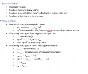
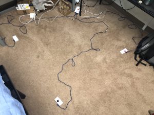
I also assembled an experimental setup to test the algorithm, setting up the tags and anchors in a 1×1 meter square. I set up two slave anchors that broadcast the time of pulse reception to the Raspberry Pi server, a master that only broadcasts a timestamp, and a stationary tag that broadcasts its ID. The setup was meant to keep both anchors 1 meter away from both the tag and the master simultaneously.
Our progress is on schedule for a demo this Wednesday. Udit and Rhea have been making substantial progress towards an effective multilateration algorithm with imperfect data, and I have established a consistent workflow for graphing and collecting timestamp data from multiple anchors and multiple tags simultaneously.
This week I will perform any final tests that Udit and Rhea need to fine-tune the multilateration algorithm, and then we will demo on Wednesday.
Rhea’s Status Update 4/12/2020
This week I worked on better understanding Kalman filters and implementing the filter in Python. I decided that since we have both a linear and and non-linear localization algorithm I was going to start by implementing linear Kalman filter, and get that working first and then move on to the extended Kalman filter. I have an implementation of Kalman filter that needs that models and covariances inputted as parameters.
While discussing Kalman filters, we decided that it may be best to use a python library instead of writing it from scratch, especially for the extended Kalman filter. Using a python library still requires us to determine what models to use and what the covariances are, so it lets us jump right to fine tuning these values and getting the best results as possible.
In the coming week I will be working on determining the best values for the state transition model, observation model, covariance of process noise, and covariance of observation noise. I hope to have the Kalman filter and then the extended Kalman filter working with our simulation by the end of the week.
Team Status Update for 04/12
The team’s progress is steady. It was disrupted slightly by the midsemester demo, but Shiva has made good progress in collecting real-world data from the Decawave tags through the Raspberry Pi. Meanwhile, Udit implemented an ideal-data multilateration program that was accurate to within one foot as desired by our original implementation metrics. He and Rhea are collaborating on the imperfect-data program now.
The most significant risk to the project is on Shiva’s end. He needs to investigate the inconsistent transmission and reception timestamps generated by the Decawave hardware. In the worst case however, the team can use the imperfect data that he already collected and use that in Udit’s multilateration program.
Neither the design nor schedule of the project have changed significantly since last week.