
This week, I worked on generating data for and training the graph detection algorithm. At first, I tried gathering data from online and from my own lecture slides, but I was not able to find a sufficient number of images (only about 50 positive examples, whereas a similar detection algorithm for faces required about 120,000 images). I used a tool called Roboflow to label the graph bounding box coordinates and use them for training, but with such few images, the model produced very poor results. For example, here was one image where several small features were identified as graphs with moderately high confidence:

Due to the lack of data and the tediousness of having to manually label the bounding box coordinates of each graph on a particular slide, I decided to generate my own data: slides with graphs on them. To ensure diversity in the data set, my code for generating the data probabilistically selects elements of a presentation such as slide title, slide color, number and position of images, number and position of graphs, text position, amount of text, font style, types of graphs, data on the graphs, category names, graph title and axis labels, gridlines, and scale. This is important because if we used the same template to create each slide, the model might learn to only detect graphs if certain conditions are met. Fortunately, part of the code I wrote to randomly generate these lecture slides – specifically, the part that randomly generates graphs – will be useful for the graph description algorithm as well. Here are some examples of randomly generated graphs:
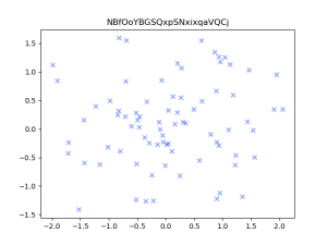
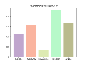
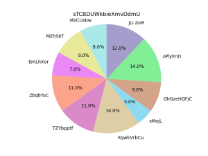
Of course, the graph generation code will have to be slightly modified for the graph description algorithm (specifically graph and axis titles) so they are meaningful and not just random strings of text; however, this should be sufficient for graph detection.
Here are some examples of the generated full lecture slides with graphs, images, and text:
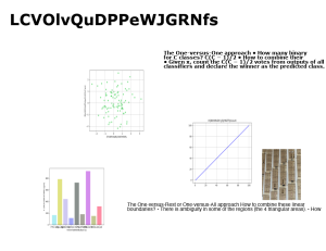
Since my code randomly chose the locations for any graphs within the slides, I easily modified the code to store these in the text file to be used as the labeled bounding box coordinates for graphs in each image.
With this, I am able to randomly generate over 100,000 images of slides with graphs, and I will train and be able to show my results on Monday.
In addition to this, I looked into how Siamese Networks are trained, which will be useful for the slide-to-image matching. I watched the following video series to learn more about few-shot learning and Siamese Networks:
I have not run many tests on the ML side yet, but I am planning to run ablation tests by varying parameters in the graph detection model, and measuring the accuracy of bounding box detection (using the loss function based on intersection over union metric) on a generated validation data set. We will also be testing the graph detection on a much smaller set of slides from our own classes, and we can provide accuracy metrics in terms of IoU for those as well. We can then compare these accuracies to those laid out in our design and use-case requirements. Similarly, for the matching algorithm, measuring accuracy is just a matter of counting up how many images were correctly vs. incorrectly matched; we will just have to separate the data we gather into training, validation, and testing sets.
My progress is almost on schedule again, but we still need to collect a lot of images for the image-slide matching, and I plan to work on this with my group next week. By next week (actually earlier, since I have completed all but the actual training), I will have the graph detection model fully completed and hopefully some results from the graph description model as well, since we are aiming to gather as many images as we can this week for that model and generate reference descriptions.