Nithya’s Status Report for 12.09.23

This week, I finalized and retrained/saved the graph detection and slide matching models, continuing to make changes to hyper parameters and values for pre-processing. The main task this week was dealing with issues in the graph description model. I was able to train the model last week and get results on input scatterplots and line graphs, and during the same run, visualize results. However, when I tried to save the model and reload it (so that we wouldn’t have to retrain every time we wanted results), I faced several issues. The root of these issues is that in Keras, only the most basic type of model (a sequential model with fully connected or convolutional layers) can be saved and loaded in this way. Since my architecture is significantly more complex and consists of a CNN followed by an encoder/decoder network, Keras would not allow me to save and reload the model with its weights after training to be used for inference.

I spent several days trying to work around this issue by looking into the Keras documentation and Stack Overflow, but in the end decided that it would be better to use a different framework for the model. I then translated all of my code into PyTorch, in which it is much easier to save and load models. I then retrained the model.

Once I did this, I also worked on the integration – I completed the slide matching integration with Aditi earlier in the week, and I worked on the graph detection and description pipeline (I had to combine them into one full system since we are using the extracted graphs from detection for the graph description). This pipeline is now complete.

I finished on schedule and all that is left for this coming week is to try to make minor tweaks to perhaps improve the slide matching accuracy further and do some user testing so that we can include results for that in our final report. We also need to finish up our final report and do some testing tomorrow of the full system before the demo.
Nithya’s Status Report for 12.2.23

There has been a lot of progress on the ML models in the last two weeks.
1.I gathered and annotated 1000 real slides from lectures with graphs to augment the dataset.
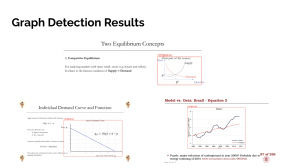
2.I trained and evaluated the graph detection model (YOLO) – this was fairly successful, but there are some small issues with the bounding box cutting off axis labels. Here are some example results.
 
3.I labeled 850 images of captured lecture slides, modified Siamese network, and trained it twice (once with class imbalance and the other with balance). This didn’t work so I switched the approach to a combined integer detection and then classification problem.
4.I wrote a script to go through all lecture PDFs and extract slides as images. I wrote another script to place the slide number in a red box in the bottom right corner of the image. There was a lot of iteration required for this in order to produce the best possible image for number detection.
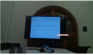
5.I gathered and annotated bounding boxes for 1000 lecture slides with the slide number in the particular format described above. I trained the object detection model YOLO to detect these slide numbers, which was successful. Here are some example results.
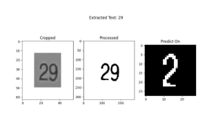
6.We tried using image processing methods such as denoising, thresholding, etc followed by tesseract (OCR) to extract the number from the cropped detected bounding box. This was not successful, so I switched to MNIST multi digit detection approach. I implemented a CNN from scratch which would classify each of the detected digits. I gathered and labeled about 600 images to augment the MNIST dataset for slide matching. I wrote a script to extract graphs from the 1000 gathered lecture slides. However the results of this were very poor, so we decided to switch back to the detection and processing approach, except using a simple MNIST classifier instead of OCR. This was fairly successful with an accuracy of 73% on a test set of 110 images from TechSpark. Here are some examples.
7.I wrote a script to generate 5000 each of line and scatter plots as well as reference descriptions.
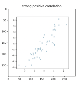
8.For graph description, I modified the CNN-LSTM code and helped write sample descriptions for the approximately 780 graphs we captured and extracted in TechSpark. Here are the results for a scatterplot:
9.I helped Aditi with integration of slide matching by compiling detection and ML models into the proper format.
We are on schedule – what still needs to be done is improving the slide matching model and simply training and evaluating the graph description model, which will be done tonight and tomorrow. We will continue to make improvements and finish the integration tomorrow.

Nithya’s Status Report for 11.18.23

This week, our entire team focused primarily on data collection for the image-slide matching model. We set up 3 different sessions for about 2 hours each in various rooms across campus and compiled a master presentation of almost 5000 unique slides to take images of using our camera. We did this in Wean, Gates, and Hamerschlag classrooms, and the images we took were also varied in terms of lighting, content of the lecture slide in the image, distance to the lecture slide, and angle. See some of these images in the team status report.


I also did some more research into the Siamese Network we will need for the image-slide matching task, particularly the loss function. One method is simple binary cross-entropy loss, where we have a training pair labelled as 1 (if the image is of the lecture slide), or 0 (if the image is different from the lecture slide). Alternatively, we can consider triplet loss. To make this work, one training example will now consist of 3 images: an anchor a (a randomly selected image from the training set – this will be a pure lecture slide), a positive example p (an image from the training set in the same class as the anchor, so an image of the same slide), and a negative example n (an image from the training set that is of a different lecture slide). We then get embeddings for each of these 3 images, and in the loss function, we want to ensure that the distance between the anchor and positive example is less than the distance between the anchor and negative example. To prevent trivial zero-embeddings or the same embeddings for all images, we will require that ||f(a) – f(p)||^2 – ||f(a) – f(n)||^2 <= -alpha, where alpha is some positive constant that we will set as a hyperparameter (note that f is the function performed on the input images by the CNN); it acts as a threshold, specifying that the distance between the anchor and positive example must be at least alpha smaller than the distance between the anchor and negative example. 


Finally, I had to go back and fix a bug from the random slide generation which was causing text to appear as rectangles on the slide. I made a Stack Overflow post to try to get help (https://stackoverflow.com/questions/77467424/getting-checkerboard-output-when-drawing-text-on-pil-image) but I ended up figuring out the problem on my own: the problem was with a specific font that I was randomly selecting, so once I removed that from the list of fonts to choose from, the problem was solved. See the team status report for some images of this.


In terms of schedule, I am a little bit behind but I think with the extra time we have next week, I will definitely be able to catch up; I will be using the extra time Wednesday – Friday to continue working on the image-slide matching model. In terms of deliverables, I hope to complete the image-slide matching model, train it using our gathered image data, and show some results here next week. 

Nithya’s Status Report for 11.11.23

This week, I worked on generating data for and training the graph detection algorithm. At first, I tried gathering data from online and from my own lecture slides, but I was not able to find a sufficient number of images (only about 50 positive examples, whereas a similar detection algorithm for faces required about 120,000 images). I used a tool called Roboflow to label the graph bounding box coordinates and use them for training, but with such few images, the model produced very poor results. For example, here was one image where several small features were identified as graphs with moderately high confidence:


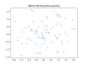
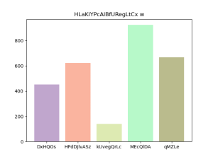
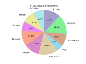
Due to the lack of data and the tediousness of having to manually label the bounding box coordinates of each graph on a particular slide, I decided to generate my own data: slides with graphs on them. To ensure diversity in the data set, my code for generating the data probabilistically selects elements of a presentation such as slide title, slide color, number and position of images, number and position of graphs, text position, amount of text, font style, types of graphs, data on the graphs, category names, graph title and axis labels, gridlines, and scale. This is important because if we used the same template to create each slide, the model might learn to only detect graphs if certain conditions are met. Fortunately, part of the code I wrote to randomly generate these lecture slides – specifically, the part that randomly generates graphs – will be useful for the graph description algorithm as well. Here are some examples of randomly generated graphs:

Of course, the graph generation code will have to be slightly modified for the graph description algorithm (specifically graph and axis titles) so they are meaningful and not just random strings of text; however, this should be sufficient for graph detection. 


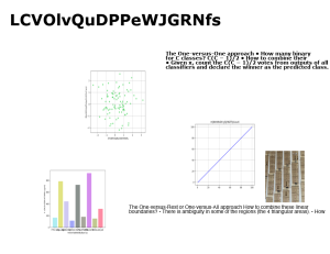
Here are some examples of the generated full lecture slides with graphs, images, and text:


Since my code randomly chose the locations for any graphs within the slides, I easily modified the code to store these in the text file to be used as the labeled bounding box coordinates for graphs in each image. 

With this, I am able to randomly generate over 100,000 images of slides with graphs, and I will train and be able to show my results on Monday. 


In addition to this, I looked into how Siamese Networks are trained, which will be useful for the slide-to-image matching. I watched the following video series to learn more about few-shot learning and Siamese Networks:

Few-Shot Learning (1/3)

Few-Shot Learning (2/3)

Few-Shot Learning (3/3)


I have not run many tests on the ML side yet, but I am planning to run ablation tests by varying parameters in the graph detection model, and measuring the accuracy of bounding box detection (using the loss function based on intersection over union metric) on a generated validation data set. We will also be testing the graph detection on a much smaller set of slides from our own classes, and we can provide accuracy metrics in terms of IoU for those as well. We can then compare these accuracies to those laid out in our design and use-case requirements. Similarly, for the matching algorithm, measuring accuracy is just a matter of counting up how many images were correctly vs. incorrectly matched; we will just have to separate the data we gather into training, validation, and testing sets. 


My progress is almost on schedule again, but we still need to collect a lot of images for the image-slide matching, and I plan to work on this with my group next week. By next week (actually earlier, since I have completed all but the actual training), I will have the graph detection model fully completed and hopefully some results from the graph description model as well, since we are aiming to gather as many images as we can this week for that model and generate reference descriptions. 


Nithya’s Status Report for 11.04.23

This week, I finished up the tutorial of the image-captioning model using the Flickr8k dataset. I decided not to train it so as to save my GPU quota for training our actual graph-description and graph identification models. 

I also looked more in depth into how image labels should be formatted. If we use a tokenizer (such as the one from keras.preprocessing.text), we can simply store all of the descriptions in the following format:


1000268201_693b08cb0e.jpg#0 A child in a pink dress is climbing up a set of stairs in an entry way .

1000268201_693b08cb0e.jpg#1 A girl going into a wooden building .

1000268201_693b08cb0e.jpg#2 A little girl climbing into a wooden playhouse .

1000268201_693b08cb0e.jpg#3 A little girl climbing the stairs to her playhouse .


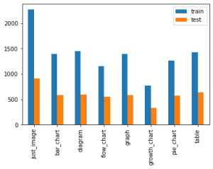
Another thought I had about reference descriptions was whether it would be better to have all reference descriptions follow the same format, or have varied sentence structure. Since the standard image captioning problem typically requires captioning a more diverse set of images (as compared to our graph description problem), there is not much guidance on tasks similar to this. Inferring from image captioning, I think that a simpler/less complex dataset would benefit from a consistent format, and this also addresses the need for precise, unambiguous descriptions (as opposed to descriptions that would be more “creative”). This is why I think we should do an ablation study where we have maybe 3 captions per each image that will differ, and then either 1) follow the same format for all images, or 2) follow a different format for each image. Here is an example of the difference on one of the images:

Ablation Case 1:

This is a bar graph. The x-axis displays the type of graph, and the y-axis displays the count for training and test data. The highest count is just_image, and the lowest count is growth_chart. 


Ablation Case 2:

This bar graph illustrates the counts of training and test graphs over a variety of different graphs, including just_image, bar_chart, and diagram. 


As you can see, the second case has more variation. We might want to have a balanced approach since we have multiple reference descriptions per image, so some of them can always have the same format, and others can have variation. 


Unfortunately, it looks like the previous Kaggle dataset we found includes graph and axis titles in a non-English language, so we will have to find some new data for that.


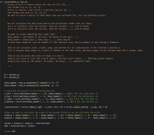
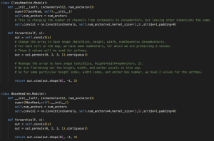
Additionally, I looked into the algorithm which will detect bounding boxes around the specific types of graphs we are interested in from a slide. I wrote some code which should be able to do this – the main architecture includes a backbone, a neck, and a head. The backbone consists of the primary CNN, which will be something like ResNet-50, and will give us feature maps. Then we can build a FPN (feature pyramid network) for the neck, which will essentially sample layers from the backbone, as well as perform upsampling. Finally, we will have 2 heads – a classification head and a regression head. 


The first head will perform classification (is this a graph or not a graph?) and the second head will perform regression to identify the 4 coordinates of the bounding box. There is also code for anchor boxes and non-max suppression (which eliminates anchor boxes with a high enough IoU, so that we are not identifying 2 bounding boxes for the same object).


Here is some of the code I worked on.


My progress is almost caught up as I got through the tutorial, but I do still need to find new graph data, generate reference descriptions with my teammates, and train the CNN-LSTM. However, I also started working on the graph detection algorithm above ahead of schedule. My plan for the next week is to work on data collection as much as possible (ideally every day with my teammates) so that I can begin training the CNN-LSTM as soon as possible. 

Nithya’s Status Report for 10.28.23

This week, I continued to work through the CNN-LSTM tutorial from last week and specifically tried to address the issue I faced last week with training. Training such large models requires GPU, and resources like Google Colab provide only a limited number of hours using the GPU for free. Since another one of my classes has assigned us many AWS credits and I am likely to have some extra, I looked into training this tutorial model (and eventually our CNN-LSTM model) on AWS. Since I was totally new to AWS, I worked through this presentation to get set up:

AWS

I learned about different Amazon Machine Images (AMIs) as well as EC2 instance types. I faced some issues launching these instances and I discovered this was because of my vCPU limits. It took several days for my limit increase request to be approved, and then I was able to launch the instance.


I also learned about persistent storage, EFS in particular. This is important because when an instance is stopped, the file storage for that instance will be deleted (and unfortunately I experienced that when I had to stop my instance and restart it). I am still having some issues working out how to set up EFS and this is something that will definitely need to be fixed before we start training our model, in order to minimize the time we need to spend paying for active instances.


My progress is still behind as I wanted to work on the graph description model this week but was still caught up with the tutorial. I did work on the tutorial several days this week but due to the delay in getting my vCPU limit increased, I did not have much time to work through the subsequent issues with EFS. For next week, I will again try to work on the tutorial and graph description model several days, and I am currently (and will continue to) look into ways to solve the EFS issue to ensure smooth training when our model is ready.


For next week, I would like to have the results of the tutorial and a draft architecture for the CNN-LSTM. I also hope to work out how to do all of the labeling/figure out how the reference captions and images should be formatted so that they can be easily fed to the model.

Nithya’s Status Report for 10.21.23

This week, I dove deeper into understanding the CNN-LSTM model and got started working with some code for one implementation of this kind of network for image captioning. I worked through the tutorial on this site:


How to Develop a Deep Learning Caption Generation Model

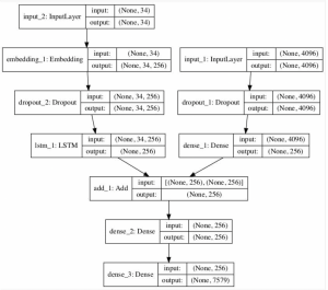
This tutorial uses images from the Flickr8k dataset. The CNN-LSTM model has 2 parts: the first is a feature extractor, and the second is the sequence model which generates the output description of the image. One important thing that I learned this week while working through this tutorial is about how the sequence model works: it generates the output sequence one word at a time by using a softmax over all words in the vocabulary, and this requires an “input sequence”, which is actually the sequence of previously generated words. Of course, we can upper-bound the length of the total output sequence (the example used 34 words as the bound).


Since the sequence model requires a “previously generated” sequence as input, we also make use of <startseq> and <endseq> tokens. Here is the example given in the article of how the CNN-LSTM would generate the description for an image of a girl:

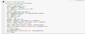
Here is a portion of the full code, which encodes the architecture of the CNN-LSTM model, as well as a diagram which is provided in the article which helped me to better understand the layers in the model. I need to do a little more research into how the feature extractor and the sequence processor are combined (the last few layers where the two branches join) using a decoder, as I didn’t fully understand the purpose of this when I read this article. This is one of the things I will be looking into next week.


I wasn’t able to train the model and test any sample images this week (the model has to train for a while and given the number of images, it would take a lot of GPU power, and my quota for this week has been exhausted) – however, this is something else I hope to do next week.


I am a little behind schedule as I was hoping to have a more comprehensive grasp of the CNN-LSTM as well as have tried out the standard version of the model (without the necessary tweaks for our use case) by this time; however, I am confident that I will be able to catch up next week, as next week is also devoted to working on the graph description model. In terms of actions I will take, I will make sure to work on the graph description model both during class-time as well as on Tuesday and Thursday to catch up.


For next week, I hope to have the test version of CNN-LSTM for image captioning fully working with some results on sample images from the Flickr8k dataset, as well as determine how to do the labelling for our gathered/generated graph data.


Nithya’s Status Report for 10.07.23

This week, I mainly worked on looking into data sources for training the graph description model. Of course, we will need a significant number of images of bar graphs, line graphs, scatterplots, and pie charts for training the graph description algorithm, even though we are planning to use pre-trained weights for the CNN-LSTM model. 


For a dataset, here is one Kaggle dataset that contains 16,000 images of graphs, separated into 8 classes – this includes bar charts and pie charts, both of which we need for our use case. It was difficult finding a source which contained scatter plots and line graphs. One alternative to trying to find a single source containing a collection of graphs is web scraping, using Beautiful Soup. Essentially, if we have a list of websites, we can write a Python script as described here (https://www.geeksforgeeks.org/image-scraping-with-python/) to extract any images from that site. We would have to manually get these URLs and also filter out any non-graph images that are found this way, but it is another way we can gather data. 


I also looked into some methods for increasing the number of images in our training set – some of these augmentation techniques are randomly cropping the image, flipping the image horizontally, changing the colors in the image, etc. Many of these, like the random crop and flipping the image, unfortunately may not be well-suited for graphs even though they are common augmentation techniques for CV tasks in general.  


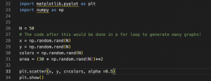
Another idea I had was to have some Python program generate graphs for us. This would be particularly useful for line and scatterplots, where a lot of the data on the x and y axes could be randomly generated using numpy. For this idea, we could also come up with a large list of axis labels so that what the graph is plotting wouldn’t be the same for all of the computer-generated graphs. Overall, I think this idea would allow us to generate a lot of varied graphs in a small amount of time, and would be a good addition to the data that we are able to gather online. 


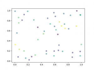
Here’s an example of what the random graph generation code would look like, as well as the resulting graph (these would be supplemented with axis labels and a title of course):


My progress is on schedule, as my goal for this week was to look into some graph data sources. For next week, my goal is to get started on understanding the code for the CNN-LSTM model, making changes to the architecture, and potentially begin training on the images of the Kaggle dataset.

Nithya’s Status Report for 09.30.23


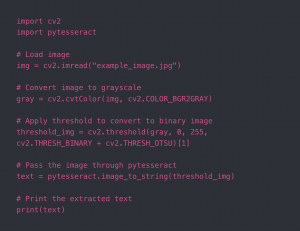
This week, I set up PyTesseract on my computer and was able to test it with a few images. Getting the tesseract module on my M1 Mac was a little challenging since certain packages are not compatible with the M1 chip (as opposed to the standard Intel chip). After getting that working, I tried running tesseract with a somewhat low quality image of my student ID card, and the results from that were fairly good, although certain parts were misidentified or left out. For example, my student ID number was correctly identified, but “Carnegie Mellon University” was read as “patnecie Mellon University”. Given that we will mainly be performing text recognition on very high quality images with our new change of pre-uploading slides, I don’t think the accuracy of PyTesseract will pose a large problem for us.  This is the code I used for testing tesseract:


I learned from visiting this site (https://tesseract-ocr.github.io/tessdoc/Data-Files-in-different-versions.html) that tesseract already has support for identifying math symbols and equations. I hope to test this out more thoroughly next week, but preliminary results from this week seemed promising (identifying numbers and symbols like = correctly). 


Since we decided to extend our use case by identifying and generating descriptions for certain types of graphs, I did a lot of research on how this would work. Initially, I looked at a few papers on the topic of “scene understanding” and “scene graph generation”, which is a similar problem to the one we are trying to solve; this involves building relationships between objects identified in images in the form of a graph. 


I went on to look at papers on the topic of image description/captioning, which I feel is the most relevant to our graph description problem. From this paper (https://aclanthology.org/P19-1654.pdf), which actually proposes a new metric for measuring how accurate descriptions of images are, I learned that there are 2 standard methods of evaluating image descriptions/captions. The first is by human judgment – ask a person to rate the overall quality of a description and also rate based on certain criteria (relevance fluency, etc.). The second is automatic metrics, which compare the candidate description to a human-authored reference description. This is typically done by Word Mover’s Distance, which measures the distance between two documents in a word embedding space. We will use the same metric for our graph descriptions. 


Courses which covered the engineering, science, and math principles our team used to develop our design include 18-240, 16-385 (Computer Vision), 18-290, 18-491 (Digital Signal Processing), 11-411 (Natural Language Processing), and 18-794 (Intro to Deep Learning & Pattern Recognition for Computer Vision). The last course in particular has already helped me a lot in understanding the different types of computer vision tasks we need to solve and the appropriate algorithms for them.


My progress is on schedule as this week, my main goal was to get PyTesseract working locally and start testing it out. Since we also made some changes to the use case, I updated my tasks in the schedule to focus more on the graph description model. 


For the next week, I want to do more research into and maybe begin implementing the first version of the matching algorithm (for matching images of slides to pre-uploaded slides). I will also begin collecting and labeling graph data with my teammates.

Nithya’s Status Report for 09.23.23

This week, I did some more research on the models for Optical Character Recognition. Here are some of the sources I looked at:

Optical Character Recognition Wiki

Tesseract GitHub 

I learned more about which algorithm specifically allow OCR to work; OCR uses a combination of image correlation and feature extraction (both of which are computer vision methods that utilize filters) to recognize characters. 

I also learned that certain OCR systems, such as Tesseract (which we mentioned in our proposal, and is open-source), use a two-pass approach. On the first pass-through, the system performs character recognition as usual, and on the second pass-through, the system actually uses the characters that it recognized with high confidence on the first pass to help predict characters that it was not able to recognize on the first pass. 

I looked into post-processing techniques for OCR, which is something we might decide to try to improve accuracy. This involves getting the extracted text and then comparing it to some kind of dictionary, acting as a sort of ‘spell check’ to correct inaccurately-recognized words. This may be harder to do if there are proper nouns which don’t appear in a dictionary, so I’d like to try an implementation with and without post-processing, and compare the accuracy. 

My progress is on schedule, as this week was meant for researching OCR models. 

For next week, I will create a small test project using Tesseract and play around with the hyperparameters and training set, in order to ascertain the current level of accuracy that this system can achieve.