Team Status Report 4/5/20

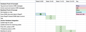
We finalized handing all the hardware we had over the Shiva and ordering more of our final hardware from Quinn to Shiva. He was able to use UART to export data from decawave radio into RPi (no longer need SPI since hardware requirement are lessened). He can now read data into the RPi and timestamp.

Shiva has MANY tests to run and data to collect. First he will use a stationary tag and stationary anchor to measure various errors and reliability. We want to see the difference between theoretical pulse transmission time differences and the differences in reception. We want to measure both the precision of the reception differences as well as the absolute difference between it and the transmission as an offset in our server code. We want to also do these tests by first timestamping in the Decawave chip and then in the raspberry Pi to see if we see which measure is more reliable. He can move on to looking at reliability with 1 stationary tag and 2 anchors and test differences in Non-LOS settings.

These experiments will be used to validate the the simulated error we will add to the hardware simulator program. If our simulator has the same percent errors as Shiva reports, we can safely validate our simulator as a way to scale our project and test the success of our Kalman smoothing and Gauss-Newton approximator.

Rhea and I have been precisely been researching and implementing those just mentioned algorithms.

We hope that we can have a basic demo with Shiva’s error graphs + Udit ideal simulation + Gauss-Newton localization by Wednesday.

Udit’s Status Report 4/5

This week’s focus was trying to fully understand the mathematical approach for my localization software.

I genuinely spent >10 hours reading papers. Based a lot of research and looking at results, I feel confident that our best approach right now is the following.

  1. Simulate player movements on a bball court in a variety of patterns and speeds (Straight line, zigzag, random, circular).
  2. Use the simulated distance between anchors and player to calculate TOAs at each anchor
  3. Send data to server program via sockets
  4. Calculate time differences (Taus) and other measurements
  5. Use the iterative Gauss-Newton method to solve the set of non-linear hyperbolic equations by least squares approximation to get (x,y) location with least residual
  6. Smooth these values by using a recursive extended Kalman filter

We are working to start off implementing this with perfect data from steps 1-2. Shiva is working on collecting experimental data from the hardware to give us an idea of high error and consistency will be in reading these numbers. We will add in simulated error based on that experimental error as our next step.

Once we get this stack working with decent success on simulations, we can replace steps 1 and 2 with the real hardware with Shiva sending packets from his simulated setup to our server code.

Step 5 is what I am in charge of and step 6 is what Rhea is in charge of.

I spent many hours reading multiple papers that offer strategies to solve the equations needed in step 5 but typos and slightly incorrect equations has slowed down the process. But here is the math I have thus far:

For each anchor i there is a (x_i, y_i) known location with an unknown (x,y) tag location.
R_i = v*T_i where v is speed of light in air and T_i is the TOF from tag to anchor i (unknown value)
tau_ij = T_i-T_j (tau is known because you can subtract timestamps)
R_i-R_j = v*T_i-v*T_j=v(T_i-T_j)=v(tau_ij)
Via algebraic manipulation, plugging in the distance formula (R_i = sqrt((x_i-x)^2+(y_i-y)^2)), and using 2 anchors as a reference, you get an equation

alpha_i*x+beta_i*y+C_i = 0 for i in {3,4} where alpha, beta and C are values calculated from v, tau_1i, x_1, y_1, x_i, y_i, tau_12, x_2, y_2 (which are all known constants or values from data).

alpha_i*x+beta_i*y+C_i = 0 for i in {3,4} gives us 2 linear equations with 2 unknowns that can be easily solved using an inverse matrix assuming perfect data. Because we don’t have perfect data, we have to use the hyperbolic equations and use a Gauss-newton least squares approximator.

I don’t fully understand the least squares method (especially how to implement it in code) and what are the exact hyperbolic equations that need to be approximated. Right now, I don’t see why we can’t estimate using the linear equation but that is my task for the next day or so.

Shiva’s Status Update for 04/05

This week, per our revised Gantt chart, I was able to send data from the Decawave chip to the Raspberry Pi over UART. Although I also wanted to transmit data over SPI, the SPI functionality in the Decawave chips were poorly documented. Their guide referenced a test program that was not actually included in the Decawave firmware and software bundle download. Thus, after conferring with my team, we decided to stick with UART over USB rather than waste time fiddling with SPI.

This week, now that I’m able to get correct timestamp data, I will be setting up a system of multiple Raspberry Pis attached to Decawave chips and collecting experimental data on metrics that can be fed into the simulator Udit and Rhea are developing.

Our team’s progress is still on schedule.

Rhea’s Status Update 4/5/2020

At the end of last week Udit suggested another paper for us to use as reference for our multilateration software.  So I started working on understanding the paper, but while going through the math I noticed that the hardware set up was different than what we have.  Instead of having a transmitting tag, and multiple receiving beacons, it had multiple transmitting beacons and receiving tag which does all the math.  We decided that moving forward with this paper would not be productive, but it helped us decide to use a Kalman filter.   We then took a look at a different paper which had a similar hardware set up to our system and used a Kalman filter.

After looking at the other paper we decided that our approach should be to use Gauss-Newton to estimate the position and then use a Kalman filter to improve the accuracy.  So I then did research on Kalman filters, to understand generally how it works, and how we might apply it to our system.

Next week I will work on implementing the Kalman filter to improve accuracy of the location we predict.